Marsh D. Applied Geometry for Computer Graphics and CAD

Подождите немного. Документ загружается.

248 Applied Geometry for Computer Graphics and CAD

9.10. Determine a NURBS sphere by rotating the NURBS circle of Exam-

ple 8.21 about the z-axis. Apply a scaling of 3 units in the x-direction

and 2 units in the y-direction to the NURBS sphere to obtain an el-

lipsoid.

9.11. Determine a NURBS representation for a torus.

9.12. (a) Apply a scaling of a units in the x-direction and b units in the

y-direction to the NURBS circle to obtain an ellipse.

(b) Assume that the ellipse lies in the z = 0 plane (by adding a zero

third coordinate to the control points). Determine a NURBS

representation of an elliptic cylinder by (i) extruding the ellipse

through 1 unit in the direction of the z-axis, and (ii) translation-

ally sweeping the line segment (1 − t)(0, 0, 0) + t(0, 0, 1) along

the trajectory curve deﬁned by the ellipse.

second coordinate to the control points). Determine a NURBS

representation of an ellipsoid (of revolution) by rotating the el-

lipse about the z-axis.

9.13. Let a hyperbola be deﬁned in NURBS form by control points

(−1, 0, 1), b

(0, 0, 0), b

(1, 0, 1), weights w

=1,w

=3,w

=1,

and knot vector −1, −1, −1, 1, 1, 1. Determine a NURBS representa-

tion of a hyperboloid (of one sheet) by rotating the hyperbola about

the z-axis.

9.14. Determine the ruled surface deﬁned by the NURBS circle B(t)(as-

sumed to be in the z = 0 plane), and the quadratic NURBS curve

with control points b

(4, 0, 3), b

(4, 2, 3), b

(−4, 2, 3), b

(−4, 0, 3),

(−4, −6, 3), b

(4, −6, 3), b

(4, 0, 3), weights 1, 1, 1/2, 1, 1/2, 1, 1,

and knot vector 0, 0, 0, 1/4, 3/4, 1, 1, 1.

9.5 Surface Subdivision

The de Casteljau, de Boor, and knot insertion algorithms for integral and ra-

tional B´ezier and B-spline curves can be applied to surfaces. For instance, to

subdivide (or to evaluate the coordinates of a point of) a B´ezier surface S(s, t)

at the parameter value (s

), the de Casteljau algorithm is applied ﬁrst in the

t direction, and then again in the s direction, or vice versa. To apply the algo-

rithm in the t direction, each row of the control polyhedron (that is, the control

points p

i,j

with ﬁxed i) is treated as the control polygon of a B´ezier curve in

9. Surfaces 249

the parameter t, and the de Casteljau algorithm is executed with t = t

.This

yields a subdivision of S(s, t)intotwoB´ezier subsurfaces along the parameter

curve S(s, t

). Similarly, the de Casteljau algorithm is executed with s = s

each column of the control polygon (that is, the control points p

i,j

with ﬁxed

j). The result is that the surfaces are subdivided along the parameter curve

S(s

,t), giving a subdivision of the original surface into four surface patches.

The algorithm also yields an evaluation of the point S(s

In a similar manner, the rational de Casteljau algorithm can be applied to

a rational B´ezier surface, and the de Boor and knot insertion algorithms can

be applied to a B-spline or NURBS surface. The following example elucidates

the method further.

Example 9.21

AB´ezier surface S(s, t) has control points

0,0

(2, 3, 0), p

0,1

(2, 6, 3), p

0,2

(2, 10, 0) ,

1,0

(6, 2, 1), p

1,1

(6, 6, 4), p

1,2

(6, 9, 1) ,

2,0

(10, 2, 0), p

2,1

(10, 6, 3), p

2,2

(10, 10, 0) .

Apply the de Casteljau algorithm to subdivide the surface along the coordinate

curves S(0.5,t)andS(s, 0.25), and to evaluate the point S(0.5, 0.25). Applying

the de Casteljau algorithm with t =0.25 to each row of control points yields

row i =0

(2, 3, 0) (2, 6, 3) (2, 10, 0)

(2.0, 3.75, 0.75) (2.0, 7.0, 2.25)

(2.0, 4.5625, 1.125)

row i =1

(6, 2, 1) (6, 6, 4) (6, 9, 1)

(6.0, 3.0, 1.75) (6.0, 6.75, 3.25)

(6.0, 3.9375, 2.125)

row i =2

(10, 2, 0) (10, 6, 3) (10, 10, 0)

(10.0, 3.0, 0.75) (10.0, 7.0, 2.25)

(10.0, 4.0, 1.125)

The result is two surfaces: the ﬁrst with control points

0,0

(2, 3, 0), p

0,1

(2.0, 3.75, 0.75) , p

0,2

(2.0, 4.5625, 1.125) ,

1,0

(6, 2, 1), p

1,1

(6.0, 3.0, 1.75) , p

1,2

(6.0, 3.9375, 2.125) ,

2,0

(10, 2, 0), p

2,1

(10.0, 3.0, 0.75) , p

2,2

(10.0, 4.0, 1.125) ,

and the second surface with control points

0,0

(2.0, 4.5625, 1.125) , p

0,1

(2.0, 7.0, 2.25) , p

0,2

(2, 10, 0) ,

1,0

(6.0, 3.9375, 2.125) , p

1,1

(6.0, 6.75, 3.25) , p

1,2

(6, 9, 1) ,

2,0

(10.0, 4.0, 1.125) , p

2,1

(10.0, 7.0, 2.25) , p

2,2

(10, 10, 0) .

250 Applied Geometry for Computer Graphics and CAD

Next, apply the de Casteljau algorithm with s =0.5 to the ﬁrst subsurface

(2, 3, 0) (6, 2, 1) (10, 2, 0)

(4, 2.5, 0.5) (8, 2, 0.5)

(6, 2.25, 0.5)

(2, 3.75, 0.75) (6, 3, 1.75) (10, 3, 0.75)

(4, 3.375, 1.25) (8, 3, 1.25)

(6, 3.1875, 1.25)

(2.0, 4.5625, 1.125) (6.0, 3.9375, 2.125) (10.0, 4.0, 1.125)

(4.0, 4.25, 1.625) (8.0, 3.96875, 1.625)

(6.0, 4.109375, 1.625)

and then to the second subsurface

(2.0, 4.5625, 1.125) (6.0, 3.9375, 2.125) (10.0, 4.0, 1.125)

(4.0, 4.25, 1.625) (8.0, 3.96875, 1.625)

(6.0, 4.109375, 1.625)

(2, 7, 2.25) (6.0, 6.75, 3.25) (10, 7, 2.25)

(4.0, 6.875, 2.75) (8.0, 6.875, 2.75)

(6.0, 6.875, 2.75)

(2, 10, 0) (6, 9, 1) (10, 10, 0)

(4.0, 9.5, 0.5) (8.0, 9.5, 0.5)

(6.0, 9.5, 0.5)

The last triangle of points of the ﬁrst subsurface is identical to the ﬁrst triangle

of the second subsurface since the subsurfaces have a common row of control

points. In practice the triangle would only be computed once, but it is included

here twice to illustrate that the surface is divided ﬁrst into two and then into

four. As before the edges of the computed triangle give the control points

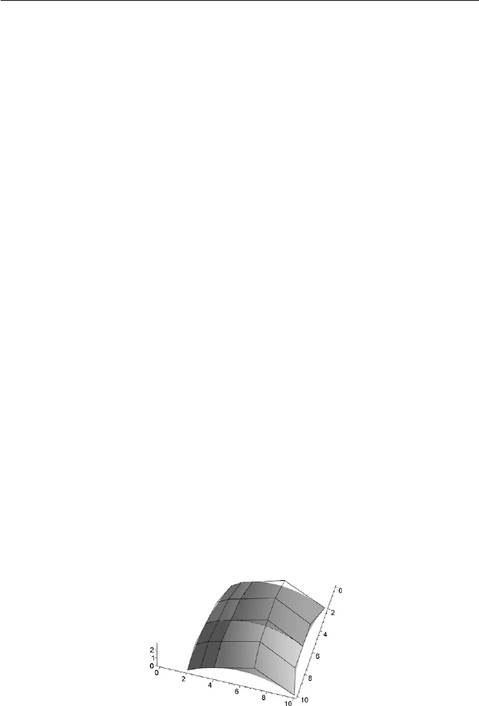
of the four surfaces resulting from the subdivision. The point S(0.5, 0.25) is

(6.0, 4.109375, 1.625). Note that only one of the t =0.25 subsurfaces needs to

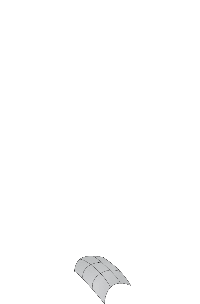
be subdivided in order to evaluate this point. The subdivided surface is shown

in Figure 9.13.

Figure 9.13 Subdivided biquadratic B´ezier surface of Example 9.21

9. Surfaces 251

Subdivision of rational B´ezier, B-spline, and NURBS surfaces is performed by

applying the rational de Casteljau, the de Boor, or a knot insertion algorithm

in a similar manner.

Remark 9.22

The number of linear interpolations computed in a subdivision of a B´ezier

surface into four is easily determined. Suppose the surface has degree m in

the s direction and degree n in the t direction. The de Casteljau algorithm

in the s direction requires

m(m + 1) interpolations for each column giving

a total of

m(m +1)(n + 1) interpolations. The algorithm in the t direction

(remembering that there are now 2m +1 rows of n control points) requires

n(n+1) interpolations per row giving

(2m +1)n(n+1) interpolations in all.

The total number of interpolations is

m(m+1)(n +1)+

(2m +1)n(n+1) =

(n +1)



2mn + n + m

+ m



. Thus, depending on the degrees m and n,it

matters which direction is subdivided ﬁrst. For instance, if m =3,n =4,then

the number of computations is 100. But if m =4,n = 3, then the number of

computations is 94. Thus it is most eﬃcient to subdivide ﬁrst in the variable

which has the largest degree.

EXERCISES

9.15. In Section 6.10.3, a method to determine the intersection of two

B´ezier curves using subdivision was described. Describe how the op-

eration of subdivision together with the convex hull property for

surfaces can be used to determine the curve of intersection of two

B´ezier surfaces.

9.16. Subdivide the B´ezier surface of Example 9.21 at s =0.25 and t =0.5.

9.17. Subdivide the B´ezier surface of Example 9.13 at s =0.4andt =0.2.

9.18. Use the de Boor algorithm to subdivide the B-spline surface of Ex-

ercise 9.3 at s =2.2andt =6.4.

9.6 Skin and Loft Surfaces

Skinning is the operation of constructing a surface that interpolates a number

of user speciﬁed curve sections. Clearly, there are an inﬁnite number of surfaces

passing through two curves c(t)andd(t). One solution is to linearly interpolate

252 Applied Geometry for Computer Graphics and CAD

the two curves to give the ruled surface

x(s, t)=(1− s)c(t)+sd(t) . (9.15)

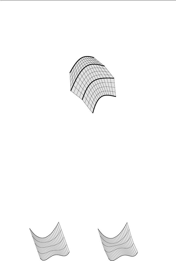
A sequence of curve sections can be skinned by computing ruled surfaces be-

tween adjacent pairs of curves as shown in Figure 9.14.

Figure 9.14 Skinning through curve sections

Example 9.23

Let two curve sections be c(t)=(t, t

, 0) and d(t)=(t, t

− t

, 10). Then the

skinning surface given by Equation (9.15) is

x(s, t)=



(1 − s)t + st, (1 − s)t

+ s(t

− t

), (1 − s)0 + s10



=(t, t

− 2st

+ st

, 10s) .

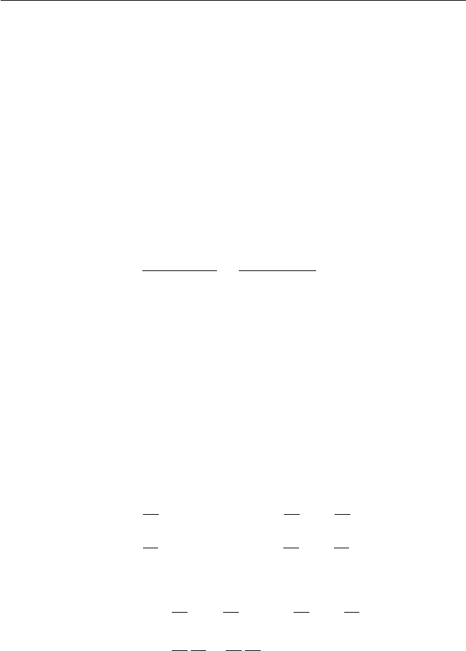
Figure 9.15(a) shows the skin surface and the intermediate parameter curves

corresponding to s =0.25, s =0.5ands =0.75.

d()t

c()t

s = 0.25

s = 0.5

s = 0.75

d()t

c()t

s = 0.25

s = 0.5

s = 0.75

(a) (b)

Figure 9.15 Skin and loft surfaces of Examples 9.23 and 9.25

9. Surfaces 253

More general skinning surfaces can be achieved by replacing the blending func-

tions 1 −s and s in (9.15) by continuous functions f

(s)andf

(s) that satisfy

(0) = f

(1) = 1 and f

(1) = f

(0) = 0. Additionally, the blending functions

can be required to satisfy f

(s)+f

(s) = 1 in order to obtain skin surfaces that

are planar whenever the boundary curves are coplanar (Exercise 9.23).

To proceed further, it is necessary to introduce the notion of geometric

continuity for surfaces in a similar manner to curves in Deﬁnition 7.14.

Deﬁnition 9.24

Two regular surfaces x(s, t)andy(u, v) are said to meet with (parametric)

-continuity at a point P = x(s

)=y(u

) whenever

∂

i+j

x(s

)

∂

s∂

∂

i+j

y(u

)

∂

u∂

for 0 ≤ i + j ≤ k.

Two regular surfaces x(s, t)andy(u, v) are said to meet with G

-continuity

at a point P = x(s

)=y(u

) whenever there is an invertible mapping

(called a reparametrization ) h :(˜u, ˜v) → (u(˜u, ˜v),v(˜u, ˜v)) such that x(s, t)and

y(u(˜u, ˜v),v(˜u, ˜v)) meet with C

-continuity at P. Two surfaces are said to meet

with G

-continuity along a curve if they meet with G

-continuity at every point

of that curve.

Suppose that x(s, t)andy(u, v) meet with G

-continuity at P = x(s

y(u

). Then there is a reparametrization u = u(˜u, ˜v), v = v(˜u, ˜v) for which

the chain rule gives

∂

∂˜u

y(u(˜u, ˜v),v(˜u, ˜v)) =

∂u

∂˜u

∂v

∂˜u

, (9.16)

∂

∂˜v

y(u(˜u, ˜v),v(˜u, ˜v)) =

∂u

∂˜v

∂v

∂˜v

. (9.17)

Hence

× x



∂u

∂˜u

∂v

∂˜u





∂u

∂˜v

∂v

∂˜v





∂u

∂˜u

∂v

∂˜v

−

∂v

∂˜u

∂u

∂˜v



× y

) .

Therefore, when two surfaces meet with G

-continuity at a point P,theyhave

the same normal directions, and hence the same tangent planes. The converse is

also true: if two surfaces meet at a point P, and have common surface normals

at P, then the surfaces meet with G

-continuity (Exercise 9.22).

254 Applied Geometry for Computer Graphics and CAD

Skinning is often referred to as lofting, a term that arises from the ship-

building industry where some aspects of ship design took place in the lofts of

hangers. Some authors reserve the term “lofting” to mean a skinning operation

where the interpolating surfaces satisfy speciﬁed derivative conditions along the

curve sections. When a skinning operation is applied to a sequence of curve sec-

tions, the resulting surfaces meet (in general) with only C

-continuity. Lofting,

however, can yield surfaces that have G

-continuity along the curve sections.

Suppose two curve sections c(t)andd(t) and two derivative functions c

(t)

and d

(t) are speciﬁed. There is no unique loft surface but a commonly used

one is

x(s, t)=H

(s)c(t)+H

(s)d(t)+

(s)c

(t)+

(s)d

(t) , (9.18)

where H

(s)and

(s) are the Hermite polynomials:

(s)=1− 3s

+2s

(s)=s − 2s

+ s

(s)=3s

− 2s

(s)=−s

+ s

Example 9.25

Let the curve sections be c(t)=(t, 0,t

)andd(t)=(t, 2,t

− t

), and the

derivative conditions be c

(t)=(0, 2, −1) and d

(t)=(0, 4, −0.5). (Note that

the derivative conditions can be non-constant.) Then the lofting surface given

by Equation (9.18) is

x(s, t)=(1− 3s

+2s

)(t, 0,t

)+(3s

− 2s

)(t, 2,t

− t

)

+(s − 2s

+ s

)(0, 2, −1) + (−s

+ s

)(0, 4, −0.5) .

The coordinate functions simplify to

x(t)=(1− 3s

+2s

)t +(3s

− 2s

)t = t,

y(t)=2(3s

− 2s

)+2(s − 2s

+ s

)+4(−s

+ s

)

=2s − 2s

+2s

z(t)=(1− 3s

+2s

+(3s

− 2s

)(t

− t

)

− (s − 2s

+ s

) − 0.5(−s

+ s

)

= −s +2.5s

− 1.5s

+ t

− 6s

+4s

+3s

− 2s

The surface is shown in Figure 9.15(b).

9. Surfaces 255

More general lofting surfaces can be obtained by replacing the blending func-

tions H

, H

and

by functions f

(s), f

(s), g

(t), g

(t)thatsatisfy

(0) = f

(1) = 1 ,f

(1) = f

(0) = 0 ,



(0) = f



(1) = 0 ,f



(0) = f



(1) = 0 ,

(0) = g

(1) = 0 ,g

(0) = g

(1) = 0 ,



(0) = g



(1) = 1 ,g



(1) = g



(0) = 0 ,

to give the surface

x(s, t)=f

(s)c(t)+f

(s)d(t)+g

(s)c

(t)+g

(s)d

(t) . (9.19)

Next consider the task of constructing a surface through four boundary

curves: c(t), d(t), e(s)andf(s), as showed in Figure 9.16. Consider the skin

-10

c()t

d()t

e( )t

f( )t

Figure 9.16 Gordon–Coons surface interpolating four boundary curves

surface x(s, t) that interpolates c(t)andd(t) given by (9.15). Substituting t =0

into (9.15) gives

x(s, 0) = (1 − s)c(0) + sd(0) .

Therefore, in order for x(s, t) to interpolate e(s)whent = 0 it is necessary to

modify (9.15) by adding

e(s) − (1 − s)c(0) − sd(0) .

Similarly, substituting t = 1 into (9.15) gives

x(s, 1) = (1 − s)c(1) + sd(1) ,

andinorderforx(s, t) to interpolate f(s)whent = 1 it is necessary to modify

(9.15) by adding

f(s) − (1 − s)c(1) − sd(1) .

256 Applied Geometry for Computer Graphics and CAD

The necessary correction across the entire surface is obtained by linearly inter-

polating the two correction terms

(1 − t)(e(s) − (1 − s)c(0) − sd(0)) + t (f(s) − (1 − s)c(1) − sd(1)) . (9.20)

Subtracting (9.20) from (9.15) yields the Gordon–Coons surface

x(s, t)=(1− s)c(t)+sd(t)+(1− t)e(s)+tf(s)

− (1 − s)(1 − t)x

0,0

− (1 − s)tx

0,1

− s(1 − t)x

1,0

− stx

1,1

(9.21)

where

0,0

= c(0) = e(0) , x

0,1

= c(1) = f(0) ,

1,0

= d(0) = e(1) , x

1,1

= d(1) = f(1) .

The Gordon–Coons surface can be expressed in matrix form

x(s, t)=



1 − ss1



⎛

⎝

−x

0,0

−x

0,1

c(t)

−x

1,0

−x

1,1

d(t)

e(s) f(s) 0

⎞

⎠

⎛

⎝

1 − t

⎞

⎠

. (9.22)

The reader should verify that an identical formula is obtained if the above

method is applied to the interpolant of e(s)andf(s).

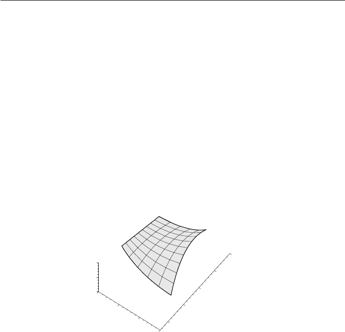
Example 9.26

Consider four boundary B´ezier curves that meet at vertices x

0,0

(−4, 0, −4),

0,1

(20, 0, 4), x

1,0

(−8, 20, 0) and x

1,1

(28, 30, 6) given by

c(t)=(−4, 0, −4)(1 − t)+(20, 0, 4)t,

d(t)=(−8, 20, 0)(1 − t)

+(10, 22, 16)2(1 − t)t +(28, 30, 6)t

e(s)=(−4, 0, −4)(1 − s)

+(−7, 12, −8)2(1 − s)s +(−8, 20, 0)s

f(s)=(20, 0, 4)(1 − s)

+(25, 12, 1)2(1 − s)s +(28, 30, 6)s

Using (9.21), the Gordon–Coons surface is x(s, t)=(x(s, t),y(s, t),z(s, t))

9. Surfaces 257

where

x(s, t)=4(1− s)(1− t) − 20 (1 − s) t +8s (1 − t) − 28 st

+(1− s)(−4+24t)+s



−8(1− t)

+20(1− t) t +28t



+(1− t)



−4(1− s)

− 14 (1 − s) s − 8 s



+ t



20 (1 − s)

+50(1− s) s +28s



= −4+24t − 6 s +16st +2s

− 4 ts

y(s, t)=−20 s (1 − t) − 30 st + s



20 (1 − t)

+44(1− t) t +30t



+(1− t)



24 (1 − s) s +20s



+ t



24 (1 − s) s +30s



=24s − 6 st +6st

− 4 s

+10ts

z(s, t)=4(1− s)(1− t) − 4(1− s) t − 6 st +(1− s)(−4+8t)

+ s



32 (1 − t) t +6t



+(1− t)



−4(1− s)

− 16 (1 − s) s



+ t



4(1− s)

+2(1− s) s +6s



= −4+8t − 8 s +28st − 26 st

+12s

− 4 ts

The surface is shown in Figure 9.16.

Given a grid or network of curves, as showed in Figure 9.17, Gordon–Coons

surfaces can be used to skin between each set of four boundary curve segments

to give a C

network surface. A general Gordon–Coons surface can be obtained

by replacing the blending functions 1 −s, s,1−t, t, that are used in (9.22), by

functions f

(s), f

(s), g

(t), g

(t)thatsatisfy

(0) = g

(0) = 1,f

(s)+f

(s)=1,

(1) = g

(1) = 0,g

(t)+g

(t)=1.

Figure 9.17 Network of curves interpolated by Gordon–Coons surfaces