Marsh D. Applied Geometry for Computer Graphics and CAD

Подождите немного. Документ загружается.

8. B-splines 207

EXERCISES

8.12. Apply the de Boor algorithm to evaluate the uniform B-spline of

Example 8.8 at t =2.5andt =4.2.

8.13. An open B-spline B(t)ofdegreed = 2 is deﬁned on the knot vector

=0,t

=1,t

=2,t

=3,t

=3,

and with control points b

(1, 1), b

(3, 4), b

(6, 2), b

(4, 2), b

(2, 5).

Apply the de Boor algorithm to evaluate the point B(2.4).

8.14. Let B(t) be a B-spline of degree d deﬁned on the knot vector t

for i =0,...,d,andt

= 1 for i = d +1,...,2d + 1. Show that the

de Boor algorithm specializes to the de Casteljau algorithm (that is,

= t). Deduce that any B-spline curve deﬁned on this knot vector

is a B´ezier curve of degree d.

8.15. Let N

i,d

(t) be the B-spline basis functions of degree d deﬁned on the

knot vector t

= 0 for i =0,...,d,andt

=1fori = d+1,...,2d+1.

Show that N

i,d

(t) are the Bernstein basis functions and deduce that

any B-spline curve deﬁned on this knot vector is a B´ezier curve of

degree d.

8.16. Implement the de Boor algorithm and verify your solutions to the

above exercises.

8.1.6 Derivatives of a B-spline

The next aim is to determine the derivative of a B-spline curve of degree d as

a B-spline of degree d − 1. The ﬁrst step is to determine the derivatives of the

basis functions of degree d in terms of the basis functions of degree d − 1.

Lemma 8.14

The derivative of the B-spline basis functions N

i,d

(t)ofdegreed may be ob-

tained in terms of the basis functions of degree d − 1 as follows:



i,d

(t)=

i+d

− t

i,d−1

(t) −

i+d+1

− t

i+1

i+1,d−1

(t) . (8.11)

Proof

The proof is by induction on d. The initial induction step (d =1)



i,1

(t)=

i+1

−t

i,0

(t) −

i+2

−t

i+1

i+1,0

(t) ,

208 Applied Geometry for Computer Graphics and CAD

is left as an exercise to the reader. Next, suppose that (8.11) is true for all

B-splines of degree d. It is necessary to show that (8.11) is true for B-splines

of degree d + 1. The recursive deﬁnition of the B-spline basis functions gives

i,d+1

t−t

i+d+1

−t

i,d

(t)+

i+d+2

−t

i+d+2

−t

i+1

i+1,d

(t) .

The derivative is obtained by applying the product rule,



i,d+1

(t)=

i+d+1

−t

i,d

(t)+

t−t

i+d+1

−t



i,d

(t)

−

i+d+2

−t

i+1

i+1,d

(t)+

i+d+2

−t

i+d+2

−t

i+1



i+1,d

(t) .

Since N



i,d

(t)andN



i+1,d

(t) are derivatives of basis functions of degree d,the

induction hypothesis (8.11) can be applied to give



i,d+1

(t)

i+d+1

−t

i,d

(t)+

t−t

i+d+1

−t



i+d

−t

i,d−1

(t) −

i+d+1

−t

i+1

i+1,d−1

(t)



−

i+d+2

−t

i+1

i+1,d

(t)+

i+d+2

−t

i+d+2

−t

i+1



i+d+1

−t

i+1

i+1,d−1

(t)

−

i+d+2

−t

i+2

i+2,d−1

(t)



i+d+1

−t

i,d

(t) −

i+d+2

−t

i+1

i+1,d

(t)+

d(t−t

)

i+d+1

−t

)(t

i+d

−t

)

i,d−1

+ d



i+d+2

−t)

i+d+2

−t

i+1

)(t

i+d+1

−t

i+1

)

−

(t−t

)

i+d+1

−t

)(t

i+d+1

−t

i+1

)



i+1,d−1

− d

i+d+2

−t)

i+d+2

−t

i+1

)(t

i+d+2

−t

i+1

)

i+2,d−1

But

i+d+2

−t

i+d+2

−t

i+1

−

t−t

i+d+2

−t

i+d+1

−t

i+d+1

−t

−

t−t

i+1

i+d+2

−t

i+1

Hence,



i,d+1

(t)=

i+d+1

−t

i,d

(t) −

i+d+2

−t

i+1

i+1,d

(t)

i+d+1

−t



t−t

i+d

−t

i,d−1

(t) −

i+d+1

−t

i+d+1

−t

i+1,d−1

(t)



−

i+d+2

−t

i+1



t−t

i+1

i+d+1

−t

i+1

i+1,d−1

(t) −

i+d+2

−t

i+d+2

−t

i+1

i+2,d−1

(t)



i+d+1

−t

i,d

(t) −

i+d+2

−t

i+1

i+1,d

(t)+

i+d+1

−t

i,d

(t)

−

i+d+2

−t

i+1

i+1,d

(t)

d+1

i+d+1

−t

i,d

(t) −

d+1

i+d+2

−t

i+1

i+1,d

(t).

The ﬁnal equation has the desired form. Hence by induction the hypothesis

(8.11) is true.

It is now possible to prove the continuity property of Theorem 8.5.

8. B-splines 209

Lemma 8.15

If the interior knot t

has multiplicity p

,thenN

i,k

(t)isC

k−p

at t = t

,and

∞

elsewhere.

Proof

Since the basis functions are piecewise polynomial of degree k,theyareC

∞

everywhere except at the joins of the segments which occur at the interior

knots. Suppose t

has multiplicity p

(1 ≤ p

≤ k). The proof is by induction.

For the initial induction step, k =1,p

=1and

i,1

(t)=

t−t

i+1

−t

i,0

(t)+

i+2

−t

i+2

−t

i+1

i+1,0

(t)=

⎧

⎪

⎨

⎪

⎩

t−t

i+1

−t

, if t ∈ [t

i+1

)

i+2

−t

i+2

−t

i+1

, if t ∈ [t

i+1

i+2

)

0, otherwise.

For t = t

, N

i,1

(t)isC

∞

(and hence also C

), and since

lim

t→t

i,1

(t) = lim

t→t

−

i,1

(t)= N

i,1

)=0,

lim

t→t

i+1

i,1

(t) = lim

t→t

−

i+1

i,1

(t)=N

i,1

i+1

)=1,

lim

t→t

i+2

i,1

(t) = lim

t→t

−

i+2

i,1

(t)=N

i,1

i+2

)=0,

it follows that N

i,1

(t)isC

The induction hypothesis is that all basis functions of degree k − 1are

k−1−p

.Thensince



i,k

(t)=

i+k

− t

i,k−1

(t) −

i+k+1

− t

i+1

i+1,k−1

(t) ,

it follows that the derivatives N



i,k

(t) are expressible as sums and products of

k−1−p

functions, and therefore N



i,k

(t)isC

k−1−p

at t = t

. Hence, N



i,k

(t)

and its ﬁrst k − 1 − p

derivatives are continuous at t = t

. Thus the ﬁrst

k − p

derivatives of N

i,k

(t) are continuous at t = t

and, since N

i,k

(t) is itself

continuous, it is deduced that N

i,k

(t)isC

k−p

as required.

Theorem 8.16

The derivative of B(t)=



i=0

i,d

(t)is



(t)=

n−1



i=0

(1)

i,d−1

(t)

210 Applied Geometry for Computer Graphics and CAD

where

(1)

= d

i+1

− b

i+d+1

− t

i+1

and N

(1)

i,d−1

(t) are the degree d − 1 basis functions deﬁned on the knot vector

,...,t

m−1.

Proof

Let B(t)=



i=0

i,d

(t), t ∈ [t

m−d

], then



(t)=





i=0

i,d

(t)







i=0



i,d

(t) .

Thus (8.11) implies



(t)=



i=0

i+d

−t

i,d−1

(t) −



i=0

i+d+1

−t

i+1

i+1,d−1

(t) .

Then, since N

0,d−1

(t)=N

n+1,d−1

(t)=0fort ∈ [t

m−d

], it follows that



(t)=



i=1

i+d

−t

− b

i−1

) N

i,d−1

(t) . (8.12)

Replacing i by i + 1 in the summation, gives



(t)=

n−1



i=0

(1)

i,d−1

(t) .

As a corollary, the higher order derivatives can be obtained by repeated

applications of the lemma.

Corollary 8.17

The rth derivative of B(t)isgivenby

(r)

(t)=

n−r



i=0

(r)

i,d−r

(t)

where b

= b

(r)

=(d − r +1)

(r−1)

i+1

− b

(r−1)

i+d+1

− t

i+r

and N

(r)

i,d−r

(t) are the basis functions deﬁned on the knot vector t

,...,t

m−r.

8. B-splines 211

Example 8.18

Consider the B-spline B(t) of degree 3 deﬁned on the knot vector t

=1.2,t

1.4,t

=1.5,t

=2.0,t

=2.4,t

=3.1,t

=5.0,t

=6.4,t

=7.3, with control

points b

(2, 1), b

(4, 8), b

(5, −1), b

(3, −2), and b

(2, −4). Then the control

points of the derivative of B(t)are

(1)

− b

− t

(4, 8) − (2, 1)

1.0

=(6.0, 21.0) ,

(1)

− b

− t

(5, −1) − (4, 8)

1.6

=(1.875, −16.875) ,

(1)

− b

− t

(3, −2) − (5, −1)

3.0

=(−2.0, −1.0) , and

(1)

− b

− t

(2, −4) − (3, −2)

4.0

=(−0.75, −1.5) .

The derivative has degree d = 2, and is deﬁned on the knot vector t

=1.4,

=1.5, t

=2.0, t

=2.4, t

=3.1, t

=5.0, t

=6.4.

Example 8.19

The derivatives at the endpoints of an open B-spline of degree d are obtained

from (8.12). Set t

= t

= ···= t

and t

m−d

= t

m−d+1

= ···= t

to give





i=1

−b

i−1

i+d

−t

i,d−1

)=d

−b

d+1

−t

1,d−1

)=d

−b

d+1

−t



m−d



i=1

−b

i−1

i+d

−t

i,d−1

m−d

)=d

−b

n−1

d+n

−t

n,d−1

m−d

)

= d

−b

n−1

m−1

−t

m−d−1

thus verifying Equation (8.5).

EXERCISES

8.17. Determine the basis functions of the B-spline and its derivative of

Example 8.18.

8.18. Let a B-spline curve B(t) of degree 3 be deﬁned on the knot vector

=0.5, t

=0.8, t

=1.4, t

=2.1, t

=2.4, t

=2.9, t

=4.0,

=4.5, t

=4.9 with control points b

(−2, −3), b

(−1, 2), b

(2, 2),

(3, 0), b

(1, −3). Determine the control points of B



(t). Determine



(2.8) in the following ways.

212 Applied Geometry for Computer Graphics and CAD

(a) Determine N

(1)

i,d−1

(t) and evaluate B



(t)=



n−1

i=0

(1)

i,d−1

(t)

at t =2.8.

(b) Apply the de Boor algorithm with t =2.8 to the derivative.

8.19. Determine the control points and knots of the derivative of the B-

spline of Example 8.3. Evaluate B



(6.2) and B



(7.4) (use de Boor).

8.20. Determine the control points and knots of the derivative of the B-

spline of Example 8.7. Evaluate B



(2.5).

8.21. Determine an expression for the second derivatives at the endpoints

of an open B-spline.

8.22. Show that for k>0, the basis functions N

i,k

(t) have just one maxi-

mum value.

8.23. Implement the derivative algorithm of Theorem 8.16.

8.2 Non-uniform Rational B-Splines (NURBS)

Rational B-spline curves are obtained from (integral) B-splines in an analogous

manner to the way in which rational B´ezier curves are obtained from (integral)

B´ezier curves. They are generally referred to as NURBS which stands for Non-

Uniform Rational B-Splines.

Deﬁnition 8.20

The NURBS curve of degree d (order d + 1) with control points b

,...,b

weights w

,...,w

, and knot vector t

,...,t

, is the curve deﬁned on the

interval [a, b]=[t

m−d

]givenby

B(t)=



i=0

i,d

(t)



i=0

i,d

(t)

, (8.13)

where N

i,d

(t) are the B-spline basis functions deﬁned on the speciﬁed knot

vector, and with the understanding that if w

=0thenw

is to be replaced

by b

. The curve may also be written in the form

B(t)=



i=0

i,d

(t) ,

where

i,d

(t)=

i,d

(t)



j=0

j,d

(t)

8. B-splines 213

are the rational B-spline basis functions.

Let b

=(x

). Deﬁne homogeneous control points



), if w

=0

, 0), if w

In homogeneous coordinates the NURBS curve has the form

B(t)=



i=0

i,d

(t) .

Appropriate choices of knot vector and control points give rise to the con-

cepts of open or periodic rational B-splines. An open knot vector yields a

NURBS curve which is endpoint interpolating. A closed periodic NURBS is

obtained by choosing a periodic knot vector, repeated control points (as de-

scribed in Section 8.1.2) and a set of weights for which the ratios of the ﬁrst d

weights equal the ratios of the last d weights.

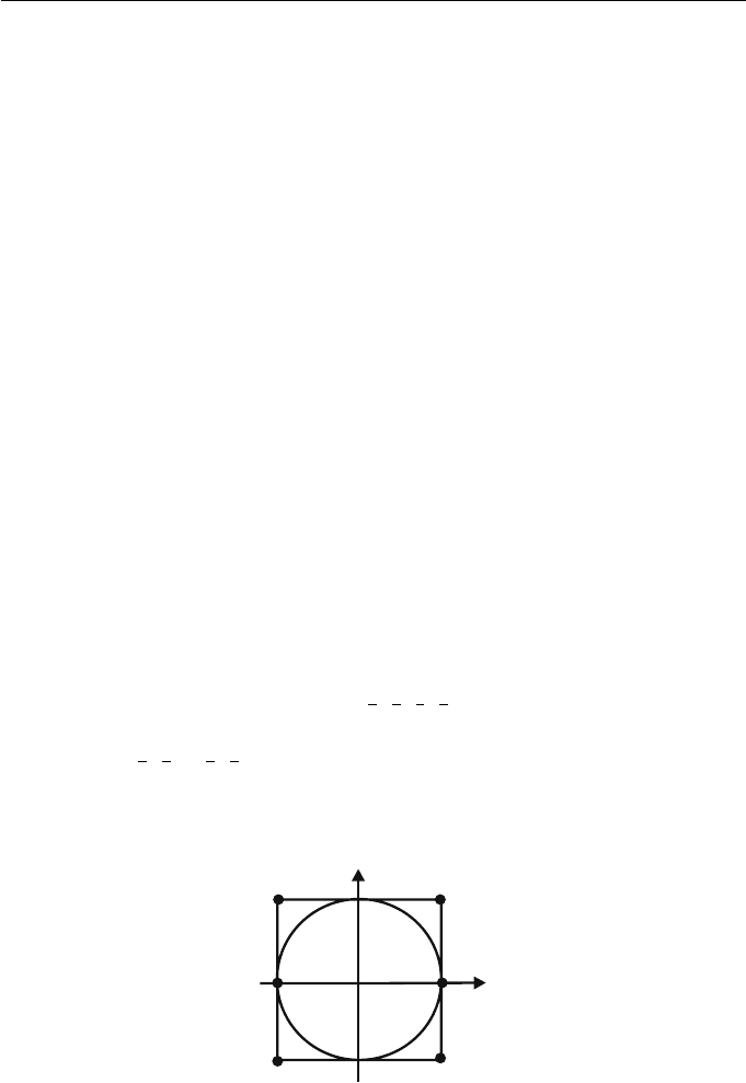
Example 8.21 (NURBS Circle)

A NURBS representation of a circle is used in the construction of surfaces

of revolution in Section 9.4.4. The unit circle centred at the origin (see Fig-

ure 8.7) can be represented by an open quadratic NURBS deﬁned on the inter-

val [0, 1]. Take the knot vector 0, 0, 0,

, 1, 1, 1, control points b

(1, 0),

(1, 1), b

(−1, 1), b

(−1, 0), b

(−1, −1), b

(1, −1), b

(1, 0), and correspond-

ing weights 1,

, 1,

, 1. Arbitrary circles and ellipses may be obtained by

applying transformations to the control points. Note that there are many ways

of obtaining a NURBS circle.

b=b

b =b

Figure 8.7 NURBS representation of a unit circle

214 Applied Geometry for Computer Graphics and CAD

Theorem 8.22

A NURBS curve B(t) given by (8.13) satisﬁes the following properties.

Local Control: If t ∈ [t

r+1

)(d ≤ r ≤ m − d − 1) then

B(t)=



i=r−d

i,d

(t)



i=r−d

i,d

(t)



i=r−d

i,d

(t) .

Convex Hull Property: If the weights w

are all positive and t ∈ [t

r+1

)

(d ≤ r ≤ m − d − 1) then B(t) ∈ CH{b

r−d

, ..., b

Continuity:Ifp

is the multiplicity of the breakpoint t = u

,thenB(t)is

d−p

(or greater) at t = u

and C

∞

elsewhere.

Invariance under Aﬃne Transformations:LetT be an aﬃne transfor-

mation. Then





i=r−d

i,d

(t)



i=r−d

i,d

(t)





i=r−d

T (b

) N

i,d

(t)



i=r−d

i,d

(t)

Invariance under Projective Transformations:LetT be a projective

transformation. Then





i=0

i,d

(t)





i=0





i,d

(t)

where

are the homogeneous control points. See Section 8.2.1.

The analogous result to Theorem 7.25 concerning the eﬀect of changing a weight

is the following theorem. The proof is similar.

Theorem 8.23

The eﬀect of changing a weight from w

to w

∗

= w

+ δw

is that any point

b = B(t) on the curve moves in the direction of the line

−−→

(where b

is the

k-th control point).

8.2.1 Projections of NURBS Curves

The property of projective invariance is useful for the computer display of spa-

tial NURBS curves. In order to apply a projective transformation to a NURBS

8. B-splines 215

curve

B(t)=



i=0

i,n

(t)



i=0

i,n

(t)

it is suﬃcient to apply the projective transformation to the homogeneous con-

trol points

,where

=(w

)ifw

=0,and

=(b

, 0) if w

=0.The

transformed images of

deﬁne a NURBS curve which is the transformation

of B(t).

The proof is analogous to the equivalent result for rational B´ezier curves

given in Section 7.5.3. Suppose the projective transformation matrix M is ap-

plied to B(t)=



i=0

i,n

(t) (expressed in homogeneous coordinates). Then

B(t)M =





i=0

i,n

(t)



M =



i=0

i,n

(t)







i=0

ˆc

i,n

(t) ,

deﬁning a NURBS curve with control points and weights given by ˆc

from which the Cartesian control points and weights can be obtained. In par-

ticular, if the transformation is a perspective or parallel projection then the

projected image of a NURBS curve onto a viewplane can be executed by ap-

plying the projection to the homogeneous control points.

As for the case of rational B´ezier curves, the above argument can be adapted

to show that NURBS curves are invariant under the viewplane coordinate map-

ping VC and the device coordinate transformation DC. It follows that the whole

process of viewing a rational B´ezier curve can be executed by applying the com-

plete viewing pipeline matrix VP = M · VC · DC to the control points.

Example 8.24

Consider the perspective projection of Examples 4.7 and 7.27 onto the xy-

plane with viewpoint V(1, 5, 3). The projection matrix M and viewplane co-

ordinate matrix VC are determined in Example 7.27. The quadratic NURBS

curve, deﬁned on the knot vector t

=0,t

=1,t

=2,t

=3,

= 3, with control points b

(0, 0, 0), b

(1, 0, 0), b

(1, 0, 1), b

(1, 1, 1), and

weights 1, 2, 2, 1, has homogeneous control points

(0, 0, 0, 1),

(2, 0, 0, 2),

(2, 0, 2, 2),

(1, 1, 1, 1). Thus

⎛

⎜

⎝

⎞

⎟

⎠

M · VC =

⎛

⎜

⎝

0001

2002

2022

1111

⎞

⎟

⎠

M · VC =

⎛

⎜

⎝

6.6 −1.2 −3.0

9.6 −7.2 −6.0

14.4 −10.8 −4.0

4.8 −3.6 −2.0

⎞

⎟

⎠

Multiply the homogeneous control points through by −1 to give positive

weights. Then the image of the curve is the planar quadratic NURBS curve

216 Applied Geometry for Computer Graphics and CAD

with control points (−2.2, 0.4), (−1.6, 1.2), (−3.6, 2.7), and (−2.4, 1.8), and

weights 3, 6, 4, and 2 deﬁned on the same knot vector. Note that the work-

ing is essentially the same as for the projection of the rational B´ezier curve in

Example 7.27.

8.2.2 Derivatives of NURBS

A recursive formula to determine the derivative of a NURBS is obtained from

Equation (7.15) which determines the derivatives of a rational function. For a

NURBS

B(t)=



i=0

i,d

(t)



i=0

i,d

(t)

let f(t)=



i=0

i,d

(t)andg(t)=



i=0

i,d

(t) in (7.15). The deriva-

tives of f (t)andg(t) are obtained by applying the algorithm for computing

the derivatives of B-splines (Section 8.1.6) where the w

are considered to be

the control points of f(t), and the w

are considered to be the control points

of g(t).

Example 8.25

Consider the NURBS of degree 3 deﬁned on the knot vector t

=1.2, t

=1.4,

=1.5, t

=2.0, t

=2.4, t

=3.1, t

=5.0, t

=6.4, t

=7.3, with control

points b

(2, 1), b

(4, 8), b

(5, −1), b

(3, −2), b

(2, −4), and weights w

=1.0,

=1.5, w

=2.0, w

=1.5, w

=1.0. Then f(t)=



i=0

i,d

(t)

has control points w

=(2, 1), w

=(6, 12), w

=(10, −2), w

(4.5, −3), and w

=(2, −4). Thus f



(t)isdeﬁnedbycontrolpoints

(1)

− w

− t

3((6, 12) − (2, 1))

2.4 − 1.4

=(12.0, 33.0) ,

(1)

− w

− t

3((10, −2) − (6, 12))

3.1 − 1.5

=(7.5, −26.25) ,

(1)

− w

− t

3((4.5, −3) − (10, −2))

5.0 − 2.0

=(−5.5, −1.0) ,

(1)

− w

− t

3((2, −4) − (4.5, −3))

6.4 − 2.4

=(−1.875, −0.75) .