Malomed B.A. Soliton Management in Periodic Systems

Подождите немного. Документ загружается.

2.6. COLLISIONS BETWEEN SOLITONS

0.2S

o.z

cO.15

1 0.1

0.05

' \

&oMi

mmmfiatl

^sh&d'.

Midylk^l

•^.^v.

'^ ^ •^. ^

1.2 1

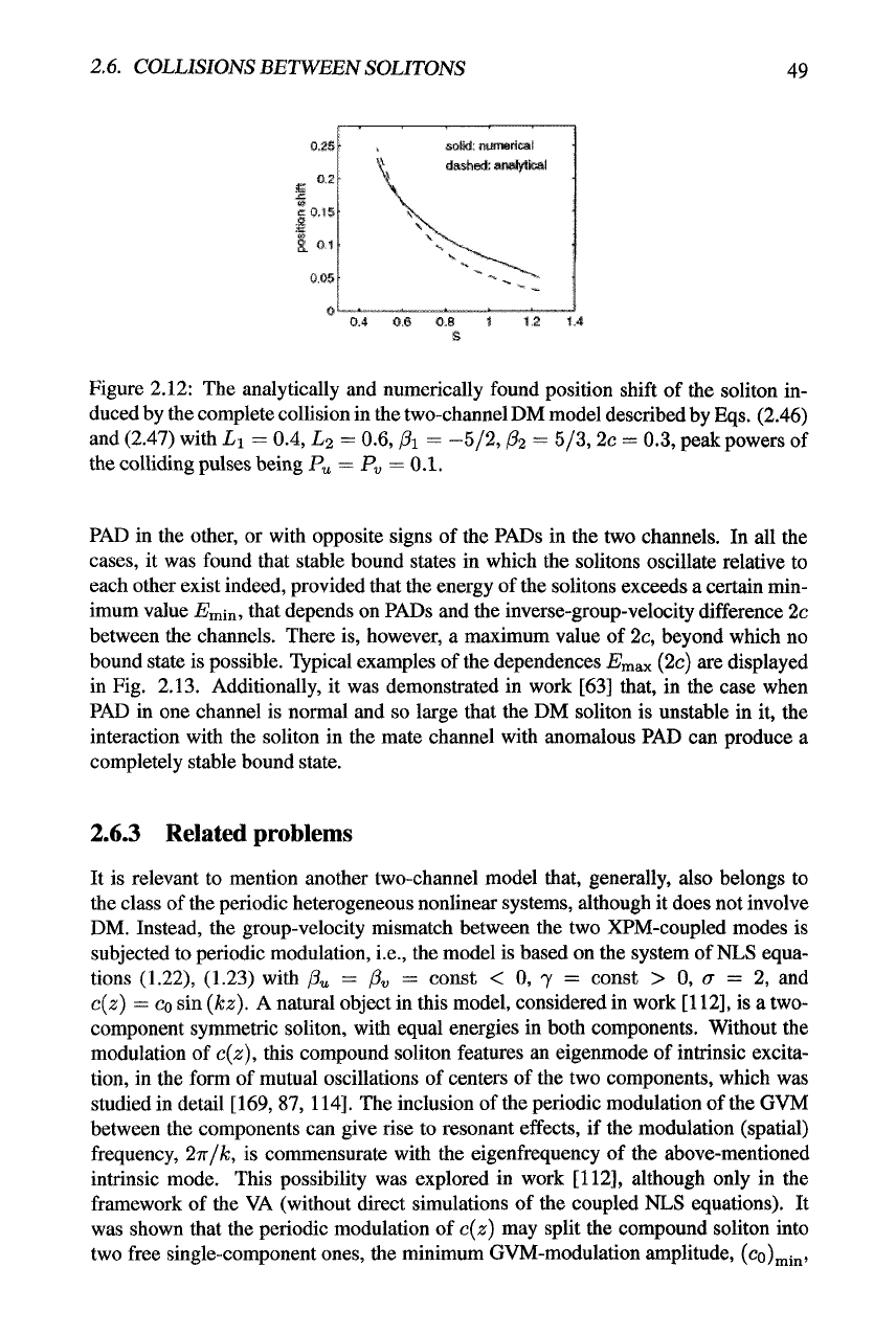
Figure 2.12: The analytically and numerically found position shift of the soliton in-

duced by the complete collision in the two-channel DM model described by

Eqs.

(2.46)

and (2.47) with Li = 0.4, Lg = 0.6, /3i = -5/2,02 = 5/3, 2c = 0.3, peak powers of

the colliding pulses being Pu = Pv = 0.1.

PAD in the other, or with opposite signs of the PADs in the two channels. In all the

cases,

it was found that stable bound states in which the solitons oscillate relative to

each other exist indeed, provided that the energy of the solitons exceeds a certain min-

imum value jBmin, that depends on PADs and the inverse-group-velocity difference 2c

between the channels. There is, however, a maximum value of 2c, beyond which no

bound state is possible. Typical examples of the dependences Emax (2c) are displayed

in Fig. 2.13. Additionally, it was demonstrated in work [63] that, in the case when

PAD in one channel is normal and so large that the DM soliton is unstable in it, the

interaction with the soliton in the mate channel with anomalous PAD can produce a

completely stable bound state.

2.6.3 Related problems

It is relevant to mention another two-channel model that, generally, also belongs to

the class of the periodic heterogeneous nonlinear systems, although it does not involve

DM. Instead, the group-velocity mismatch between the two XPM-coupled modes is

subjected to periodic modulation, i.e., the model is based on the system of

NLS

equa-

tions (1.22), (1.23) with /3„ = /?„ = const < 0, 7 = const > 0, cr = 2, and

c{z) =

sin (kz). A natural object in this model, considered in work

[112],

is a two-

component synunetric soliton, with equal energies in both components. Without the

modulation of c{z), this compound soliton features an eigenmode of intrinsic excita-

tion, in the form of mutual oscillations of centers of the two components, which was

studied in detail [169, 87, 114]. The inclusion of the periodic modulation of the GVM

between the components can give rise to resonant effects, if the modulation (spatial)

frequency, 2n/k, is commensurate with the eigenfrequency of the above-mentioned

intrinsic mode. This possibility was explored in work

[112],

although only in the

framework of the VA (without direct simulations of the coupled NLS equations). It

was shown that the periodic modulation of c{z) may split the compound soliton into

two free single-component ones, the minimum GVM-modulation amplitude,

{co)„iin'

DISPERSION MANAGEMENT

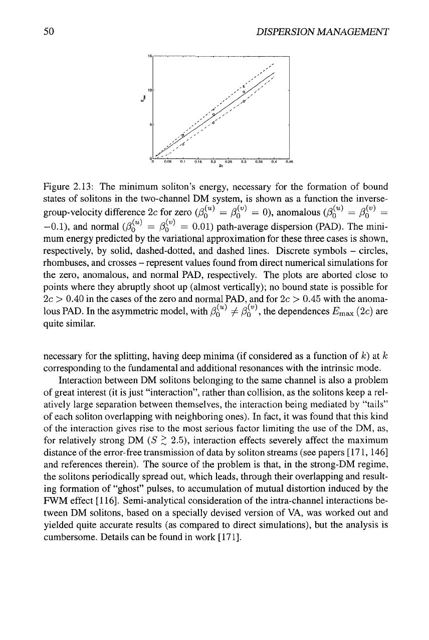
Figure 2.13: The minimum soliton's energy, necessary for the formation of bound

states of solitons in the two-channel DM system, is shown as a function the inverse-

group-velocity difference 2c for zero

(/3^"^

(3^^'

= 0), anomalous

{(3^

-0.1),

and normal

(J3Q

(u)

^'o

(v)

0.01) path-average dispersion (PAD). The mini-

mum energy predicted by the variational approximation for these three cases is shown,

respectively, by solid, dashed-dotted, and dashed lines. Discrete symbols - circles,

rhombuses, and crosses - represent values found from direct numerical simulations for

the zero, anomalous, and normal PAD, respectively. The plots are aborted close to

points where they abruptly shoot up (almost vertically); no bound state is possible for

2c> 0.40 in the cases of the zero and normal PAD, and for 2c > 0.45 with the anoma-

lous PAD. In the asymmetric model, with

(SQ

, the dependences Emax (2c) are

quite similar.

necessary for the splitting, having deep minima (if considered as a function of k) at k

corresponding to the fundamental and additional resonances with the intrinsic mode.

Interaction between DM solitons belonging to the same channel is also a problem

of great interest (it

just "interaction", rather than collision, as the solitons keep a rel-

atively large separation between themselves, the interaction being mediated by "tails"

of each soliton overlapping with neighboring ones). In fact, it was found that this kind

of the interaction gives rise to the most serious factor limiting the use of the DM, as,

for relatively strong DM {S > 2.5), interaction effects severely affect the maximum

distance of the error-free transmission of data by soliton streams (see papers [171,146]

and references therein). The source of the problem is that, in the strong-DM regime,

the solitons periodically spread out, which leads, through their overlapping and result-

ing formation of "ghost" pulses, to accumulation of mutual distortion induced by the

FWM effect

[116].

Semi-analytical consideration of the intra-channel interactions be-

tween DM solitons, based on a specially devised version of VA, was worked out and

yielded quite accurate results (as compared to direct simulations), but the analysis is

cumbersome. Details can be found in work

[171].

Chapter 3

The split-step model

3.1 Introduction to the model

The most common numerical algorithms used for simulations of equations (and sys-

tems of equations) of the NLS type belong to the "split-step" type. It is based on

splitting each step /S.z of the numerical integration, A2 =

A^AT

-|-

AZ£),

that only

the nonlinear term(s) in the equation(s) are taken into regard at the first substep, and

only the GVD and other (if any) linear term(s) are dealt with at the second substep. At

the latter stage, the corresponding linear equation(s) are solved by means of

the

Fourier

transform.

The split-step model (SSM), which was introduced in work [50] and further de-

veloped in paper [52], is formally similar to the split-step numerical algorithm, but

the difference is that the propagation distances corresponding to AZAT and Az£) are

not small, both being comparable to the soliton's period, see Eq. (1.16) (for this rea-

son, they are denoted below as Ljv and LD, respectively, rather than as AzAr,£))- In

other words, the SSM assumes periodic alternation of long segments of two different

fiber species that are (in the first approximation) purely nonlinear and dispersive, re-

spectively. Moreover, the nonlinear and dispersive components of the SSM are not

necessarily fibers - the former may be SHG (x^^^) modules [54], and the latter may be

realized as short pieces of a fiber Bragg grating. Clearly, the SSM also belongs to the

general class of the periodic heterogeneous nonlinear systems, and it is interesting to

understand if SSM can support robust solitons.

SSM has something in common with previously studied fiber-optic schemes us-

ing the so-called comb-like dispersion profile, that assumes short segments of high-

dispersion fiber inserted in a low-dispersion bulk fiber

[161].

However, there is strong

difference of SSM from the "comb" schemes: in the latter case, a large number (~ 8)

of strong-dispersion segments are inserted (non-uniformly) per dispersion length, with

the objective to emulate a continuous exponentially decreasing dispersion profile, ad-

justed to the gradual decay of the soliton's energy due to the fiber loss (so that the

soliton does not feel the system's heterogeneous structure, and its temporal width re-

mains nearly constant). On the contrary, the SSM typically assumes one dispersive and

52 SPLIT-STEP MODEL

one nonlinear sections per dispersion length, and the transmission regime is completely

different from that in the comb systems.

SSM offers a potential for applications to optical telecommunications. On the one

hand, periodically inserting short strongly nonlinear elements can help to upgrade a

linear fiber-optic link, making it possible to transmit solitons through it. On the other

hand, periodic insertion of strong dispersive elements can be useful to improve pulse

transmission in links using dispersion-shifted fibers (ones with a small value of the

GVD coefficient), where the nonlinearity may be too strong versus the dispersion.

3.2 Solitons in the split-step model

3.2.1 Formulation of the model

The dispersive segment of the SSM is described by the linear version of the NLS equa-

tion (1.5), iuz +

{1/2)UTT

= —iaou, where the GVD coefficient is normahzed to be

/? =

—1

(in the case of normal dispersion in the dispersive segments, /? > 0, the SSM

supports no solitons), and a^ is the loss constant of the dispersive fiber (in physical

units,

typical values of/? and ajj in standard telecommunication fibers are

—20

ps^/km,

and 0.2 dB/km, respectively). The substitution of u{z, r) = v{z, r) exp

{—aoz)

leads

to the lossless equation for the dispersive segment,

iVz + -Vrr = 0, (3.1)

that can be solved by the Fourier transform in r.

In the nonlinear segment, one is dealing with the dispersionless version of equation

(1.5),

iUz + \u\ u =

—iaNU,

(3.2)

where the nonlinearity coefficient is normalized to be 7 = 1 (its typical physical value

in optical fibers is 2 (Wkm)"^), and

QJAT

is the respective loss parameter. An obvious

solution to Eq. (3.2) is

u(z, T) = u(0, T) exp I —ajv z + i '• [1

—

exp

(—2af^z)]

] . (3.3)

V 2Q;iv /

In the lossless limit, a^ -^ 0, it takes the form

U{Z,T)

=u{0,T)exp{i\u{0,T)\'^z). (3.4)

It is assumed, as usual, that the losses are compensated by linear amplifiers which

act on the wave field so that

U{T) -^ U{T)

•

e^ , (3.5)

where G is the gain (in applications, the gain is usually measured in dB (deciBells),

which will be 8.696"). The value of the gain is selected so that to provide for the

balance with the total loss,

G =

LNCHN

+ LoOiD, (3.6)

3.2. SOLITONS IN THE SPLIT-STEP MODEL 53

where LD and Ljv are lengths of the periodically alternating dispersive and nonlinear

segments. In fact, the model is equivalent to its lossless version {ao = cnjv = G = 0)

with a renormalized value of Lj\f. Indeed, comparing Eqs. (3.3) and (3.4), and taking

Eqs.

(3.5) and (3.6) into regard, it is easy to see that the model including the losses and

gain is tantamount to the lossless one with LN replaced by

-(eff)

(2ajv)"^

[(1 -

6-'^°"''°)

+ e2G-2"N^o fl _ g-2a„(Ljv-zo)\| ^ (37^

where

is the distance from the beginning of the nonlinear segment to the point at

which the amplifier is installed. For this reason, in what follows below only the lossless

model is considered, making no distinction between L^^ ' and LN, nor between u and

V, see Eq. (3.1). Dynamical invariants of the lossless SSM are the same energy and

momentum as defined above in Eqs. (1.9) and (1.10). In the absence of losses, Eqs.

(3.1) and (3.2) are invariant with respect to the transformations, respectively

r -» T/KD, Z -^ z/K]^,

u -^ ANU, Z -> z/A% (3.8)

with arbitrary rescaling factors A75 and AN- This transformation may be used to set,

for instance, LN = LD = 1/2, so that the full size of the system's cell is L = 1.

The exact definition of the cell is an interval between midpoints of two neigh-

boring nonlinear segments, with a dispersive segment inserted between them. A full

transformation (map) of the pulse passing the system's cell can be represented as a su-

perposition of two transformations (3.4) corresponding to the nonlinear half-segments

at edges of the cell, and the linear transform between them, corresponding to the dis-

persive segment in the middle of the cell. Numerical simulations of the pulse evolution

in the SSM are performed by many iterations of the map, with a fixed cell's size in the

case of the regular system (or with the values of the size picked randomly from a finite

interval for a random SSM, see below).

Note that averaged (in z) version of both the regular and random SSM systems

amounts to the usual NLS equation,

2lU^ + -Urr +

\u\'^U

= 0 (3.9)

For this reason, it is natural to start the simulations with an initial pulse which would

be a fundamental soliton of the average equation (3.9),

UO(T)

= 77sech(?7r), (3.10)

with an arbitrary amplitude

rj.

Besides that, in order to understand the operation of

the system in the general case, initial pulses with an arbitrary relation between the

amplitude and width will also be considered,

uo(r) =77sech(^||jj , (3.11)

where M^ is a relative width parameter. Note that, in the case of the ordinary NLS

equation, an asymptotic (for z ^ oo) form of the solution generated by the generic

54 SPLIT-STEP MODEL

initial pulse (3.11) can be found in an exact form for any value of W

[154].

With

the GVD and nonlinearity coefficients fixed as in Eqs. (3.2) and (3.1), and with the

above normalization,

Ljsr

= LD = 1/2, free remaining parameters of the model are

the amplitude

and relative width W of the initial pulse (3.11).

It should also be noted that, while the dispersive equation (3.1) is invariant with

respect to the Galilean transformation

(1.6),

the nonlinear equation (3.2) is not formally

Galilean-invariant; however, it is obvious that the system as a whole is invariant with

respect to a modified boost transformation,

u{z, T)

I—>

u{z, T

—

cz) exp

(—c^i^/2

+ icr) , (3.12)

where 2 is the distance passed only in the dispersive segments. As well as in the case

of the ordinary NLS equation, the effective Galilean invariance of the SSM is related

to the conservation of the momentum (1.10).

3.2.2 Variational approximation

To apply the variational approximation (VA) to SSM solitons, the usual ansatz (2.6)

can be used, and, in the nonlinear segment, Eqs. (2.10) - (2.13) yield the following

evolution equations for the width and chirp:

db__2Eda_dE_

TT^

dz ' dz

(here, as above, the definition of the energy is £^ = A^a). In the dispersive segment,

the variational equations amount to

dz"^

TT^

a^' 2a dz

As £• is a constant, a solution to Eqs. (3.13) is trivial,

a = const s flmax, Kz) =

j-^—

(-2 "

-^jv),

(3.15)

"^ '^max

where

is an arbitrary constant. A general solution to Eqs. (3.14) is simple too,

a{z) = -^ , (3.16)

Tva

min

(^<in)

+'iiz-ZD)

where

and

a„iin

are other arbitrary constants.

In terms of the VA, steady transmission of the soliton implies that its amplitude,

width, and chirp return to their original values after passing a full cell of the system. It

immediately follows from Eqs. (3.15) and (3.16) that, if

is chosen to coincide with

the midpoint of the dispersive segment, the width a{z), which takes the value Omin

at this midpoint, automatically returns to the same value at the midpoint of the next

3.2. SOLITONS IN THE SPLIT-STEP MODEL 55

dispersive segment, amin being the smallest value which the width of the pulse attains

in the course of its periodic vibrations.

According to Eq. (3.17), the soliton's chirp vanishes at the midpoint of the dis-

persive segment. A condition which guarantees that it vanishes at the midpoint of the

next dispersive segment can be easily obtained: the net change of b{z) in the nonlinear

segment, which is

(^^)iV

= --5-^^iv (3.18)

" "max

according to Eq. (3.15), must exactly compensate the difference of the values of the

chirp at edges of the dispersive segment, which is, according to Eq. (3.17),

(^min)

+Lh

(to make the meaning of the expressions clearer, it is not assumed here that LD = LN)-

Note that, due to the continuity of a{z), the value a^ax which appears in Eq. (3.18) is

one attained at the edge of the dispersion segment, i.e., it is given by Eq. (3.16) with

Z- ZD =

LDJI,

flmax = • (3.20)

In fact, Omax is indeed the maximum width attained in the process of the steady propa-

gation of the SSM soliton.

Finally, the substitution of

Eqs.

(3.18), (3.20), and (3.19) into the balance condition

for b{z), (A6)^ + (A^)/) = 0, yields a basic result:

7r2(^Ey«^„ = 7r2a^,„ + L|,. (3.21)

This is a constitutive equation for the SSM solitons, which (as predicted by the VA)

determines its minimum width, ifmin. as a function of the energy E. This equation can

also be written in terms of the maximum width,

^E^ aLx = ^<ax + {LNEf . (3.22)

Considering i? as a function of

Uynm

or amax. it is easy to see that Eqs. (3.21) and

(3.22) yield exactly one physical (real) value of

amin

and exactly one value of ttmax for

any E > 0.

In the limit of LD, LN -^ 0, the SSM reduces to the average NLS equation (3.9),

with

the

extra coefficient LD/LN in front of the term (1/2)

Urr-

In this limit, the width

a{z) becomes constant, a = Amin = «max- On the other hand, the exact fundamental-

soliton solution (1.13) of the thus defined NLS equation has

(3.23)

56 SPLIT-STEP MODEL

with an arbitrary width

QQ,

the soliton's energy being E = {LD/LN)

a,o^-

Inserting

this in the limiting forms of

Eqs.

(3.21) and (3.22) corresponding to LD, LN -^ 0, one

concludes that they are satisfied automatically, i.e., the VA correctly reproduces the

exact result for the fundamental soliton in the NLS limit. The same limit corresponds

to £^

—>

0 at finite LD and LN, as in this case the soliton becomes very broad, with the

dispersion length ZD '^ cfi ^ LD, LN, hence it must be asymptotically equivalent to

the ordinary NLS soliton.

It is also relevant to note that, as it follows from Eq. (3.21), the minimum width

amin may take any value from 0 to oo when E is varied from oo to 0. However, Eq.

(3.22) shows that the maximum width Omax diverges in both limits, E ^> 0 and E -+

oo,

which suggests that there is a finite smallest value that a^ax may assume. Indeed,

analysis of

Eq.

(3.22) demonstrates that this value is (aniax)„iin ~ \/(2/7r)L£i, and it

is attained at E =

\/'1-KLDL'^.

In this case, the minimum width is (l/V2) ('^max)min-

3.2.3 Comparison with numerical results

Direct simulations of the SSM were performed in works [50, 52]. The simulations

started with the initial wave form (3.10) that would generate a fundamental soliton in

the averaged NLS equation corresponding to the SSM. In the case when the soliton

period in the averaged equation (defined as per Eq. (1.16)) is comparable to the cell's

size L, a soliton readily self-traps in the SSM, with an extremely small radiation loss

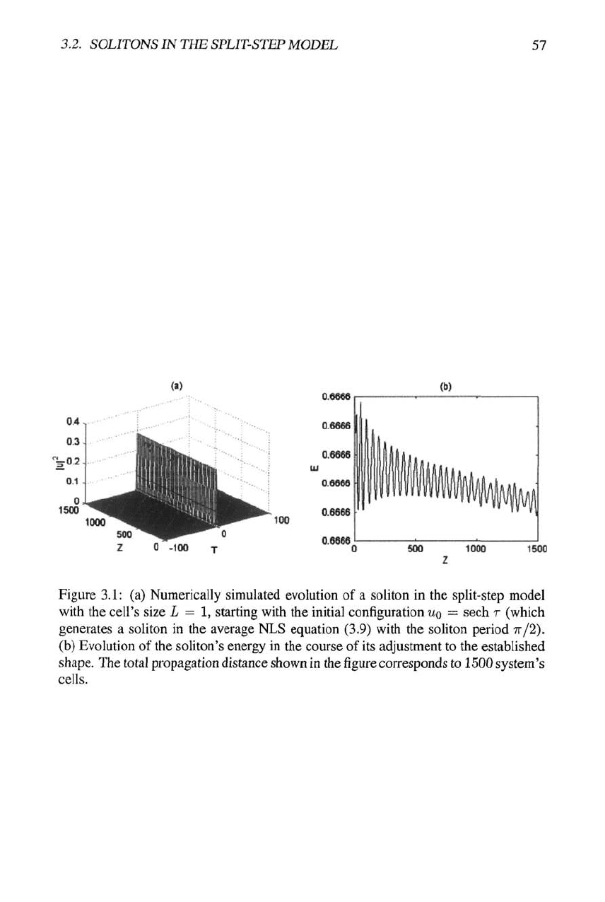
and very little change of the shape against the initial form, see an example in Fig. 3.1.

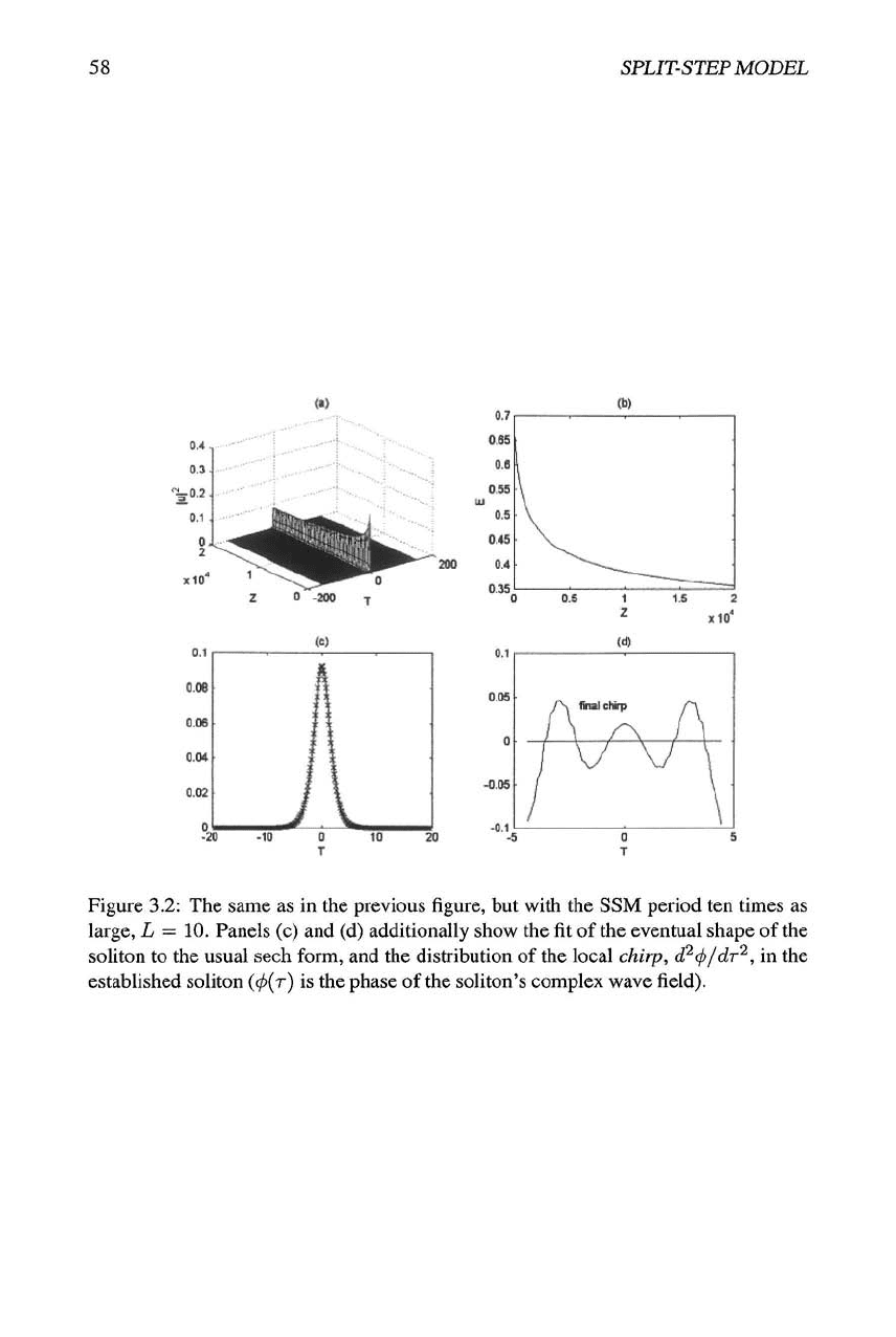
If the opposite case, with L much larger than the soliton period (with the latter de-

fined as per the average NLS equation, see Eq. (1.16)), the adjustment of the soliton

and radiation loss accompanying its relaxation to the eventual shape are quite conspic-

uous,

as shown in Fig. 3.2. In this case, the established soliton features intrinsic chirp

(i.e.,

the wave field is complex), as shown in Fig. 3.2(d). Nevertheless, the amplitude

distribution in the soliton, |'U(T)|, is still well fitted by the usual sech ansatz, see Fig.

3.2(c). In fact, the proximity of the pulse to the classical shape of the NLS soliton may

be characterized by its area,

I- + 00

A= \u{T)\dT (3.24)

(unlike the energy (1.9), the area is not a dynamical invariant of the NLS equation).

For any soliton of the average NLS equation (3.9), A = n (note that the area does not

depend on the soliton's amplitude). For the established soliton displayed in Fig. 3.2,

the area is 3.25, i.e., quite close to

TT.

If L is very large in comparison with the soliton

period in the average NLS equation, the initial pulse completely decays into radiation,

as will be explained in more detail below.

To compare the analytical results outlined above with direct simulations in a sys-

tematic way, it is more convenient to cast the constitutive equation (3.21) in a

dif-

ferent form, which determines the maximum amplitude of the SSM soliton, A^ax =

A/E/ttmin (recall that E = J^a; obviously, the largest amplitude is achieved at a point

3.2. SOLITONS IN THE SPLIT-STEP MODEL

0.4,

0.3.

-^0.2.

0.1 .

1000^^

soo

0 -100

1500

Figure 3.1: (a) Numerically simulated evolution of a soliton in the split-step model

with the cell's size L = 1, starting with the initial configuration

= sech r (which

generates a soliton in the average NLS equation (3.9) with the soliton period 7r/2).

(b) Evolution of the soliton's energy in the course of its adjustment to the established

shape. The total propagation distance shown in the figure corresponds to 1500 system's

cells.

SPLIT-STEP MODEL

Figure 3.2: The same as in the previous figure, but with the SSM period ten times as

large, L = 10. Panels (c) and (d) additionally show the fit of the eventual shape of the

soliton to the usual sech form, and the distribution of the local chirp, (Pcp/dr^, in the

established soliton ((^(r) is the phase of the soliton's complex wave field).