Malomed B.A. Soliton Management in Periodic Systems
Подождите немного. Документ загружается.

80 NONLINEARITY MANAGEMENT
4.3 Nonlinearity management for Bragg-grating and
nonlinear-Schrodinger solitons
4.3.1 Introduction to the problem
Gap solitons (GSs) in the model of the fiber Bragg grating (BG) with the cubic nonlin-
earity, based on Eqs. (1.27) and (1.28), and similar models constitute
a
separate class
of solitons. A principal difference between them and the NLS solitons
is
that the lat-
ter ones exists as
a
result
of
the balance between the self-focusing SPM nonlinearity
and anomalous temporal dispersion.
If
the nonlinearity
is
self-defocusing, while the
dispersion remains anomalous, bright solitons do not exist. However, the sign
of
the
nonlinearity does not matter in the BG model, as the effective dispersion (or diffrac-
tion, see below) induced by the grating includes both normal and anomalous branches,
hence either of them will be able to support solitons. The latter circumstance suggests
to consider
a
model where the nonlinearity may change its sign, and explore GSs
in
that case.
The simplest possibility to realize the sign-changing nonlinearity is to take
it
as
a
combination of cubic and quintic terms with opposite signs. This modification
of
the
standard BG model was considered in work
[20].
As well as in the case of the standard
BG system (1.27), (1.28) with the cubic nonlinearity, stationary soliton solutions of its
cubic-quintic counterpart were found in an exact analytical form, while their stability
was studied by means
of
numerical simulations.
It
was concluded that the family of
GSs in the modified system is drastically different from that in its standard counterpart:
the family splits into two disjoint subfamilies, each being dominated by one of the two
nonlinear terms of the opposite signs (in accordance with what might be expected), and
a part of each subfamily is stable.
A different possibility to study the effect
of
the sign-changing nonlinearity on the
GSs is to introduce a model with the nonlinearity being represented by the cubic term
only, whose sign changes periodically as
a
function
of
the evolution variable, i.e., the
NLM in combination with the BG. In the temporal domain, this implies that the non-
linearity must periodically change its sign
in
time, which
is
not
a
physically realistic
assumption. However, the necessary arrangement can be implemented in the spatial do-
main, i.e., for stationary light beams propagating across a layered structure in a planar
nonlinear waveguide.
4.3.2 Formulation of the model
According to what is said above, the model to be considered has the form
iu^+iu^+'r{z)(-\u\'^+ \v\'^\u
+
v = 0, (4.8)
iv^-iv^+'y{z)(-\vf
+ \u\Av
+
u = 0, (4.9)
where
z
is the propagation distance, which plays the role of the evolution variable in-
stead of time in Eqs. (1.27) and (1.28), and
x
is the transverse coordinate in the planar
4.3.
NONLINEARITYMANAGEMENT
81
layered waveguide. The form of
Eqs.
(4.8) and (4.9) implies that the carrier wave vec-
tors of the two waves, which are resonantly reflected into each other by BG, form equal
angles with the
z
axis. The reflecting scores (or ribs) which form the BG with spacing
h on the planar waveguide are oriented normally to the
z
axis, the Bragg-resonance
condition taking the form
of
Eq. (1.29). The usual diffraction
in
the waveguide
is
neglected, as
it
is assumed that BG gives rise to a much stronger artificial diffraction.
Although
Eqs.
(4.8) and (4.9) are z-dependent, they conserve the net power,
/
+ 00
{\u{x)fdx+\v{x)\^)dx.
(4.10)
-oo
The layered structure of the waveguide assumes that the Kerr coefficient 7(2) takes
positive and negative values 7+ and 7_ in alternating layers, cf. Eq. (3.29):
7(z)=|^+'
., /f
°<"<^+, (4.11)
'^
•' \ 7_, if
L+<
z <
L++L_,
^ ^
which
is
repeated periodically with the period
L =
L+
+ L-.
Using the scaling
invariance of
Eqs.
(4.8) and (4.9), one may always impose the following normalization
conditions:
L+
+
L_
= l,
L+7+
+
L_|7_|
= l.
(4.12)
Thus,
the model contains two irreducible control parameters, which may be selected
as,
e.g., L+ and 7+, while the other parameters can be found from Eqs. (4.12),
L_
=
1
-
L+,
7_ = -
(1
-
L+7+)
/
(1
-
L+). (4.13)
Note that corresponding average value of the Kerr coefficient is
7^'^V-^!^^-=2L^7^-l. (4.14)
Being interested in the sign-changing model, with 7_
<
0, the case of L+7+
<
1 will
be considered here, as it is equivalent to 7_
<
0 according to Eqs. (4.13).
Because the usual broad small-amplitude
GS
solitons (1.33) with ^ <C 1 are asymp-
totically equivalent to broad NLS solitons, it is natural to consider, parallel to the model
based on Eqs. (4.8), (4.9), also the spatial-domain NLS equation with the nonlinearity
coefficient subjected to the same periodic modulation as in Eq. (4.11),
1
2
iu^
+ -u^^
+ 7(z) |w|
w
=
0. (4.15)
Comparing the results for the gap and NLS solitons
in
the two models will be quite
helpful in realizing the generality of the conclusions presented below; besides that, the
model (4.15) is of interest in its own right.
82 NONLINEARITY MANAGEMENT
4.3.3 Stability diagram for Bragg-grating solitons
Unlike the NLS solitons, the variational approximation for the gap solitons is very
complex even without NLM
[113].
Therefore, one should rely on direct numerical
simulations of Eqs. (4.8), (4.9), with -j{z) defined as per Eqs. (4.11 ) and (4.13).
The simulations used the initial configuration (at
2;
= 0) in the form of the exact GS
solution (1.33) for the uniform medium, parameterized by 9 and taken at i = 0. The
simulations were run for a fixed value of 9, while the model's control parameters 7+
and L+ were gradually varied, subject to the above-mentioned constraint I'+7+ < 1.
Then, the same was done for other values of 9.
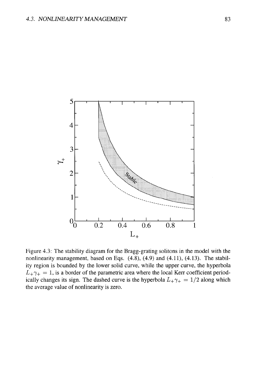
Numerical results identify a stability region for the solitons in the parameter plane
(L-I-,
7+) which is shown in Fig. 4.3. The upper boundary of the stability region is
L4.7+ = 1, which, as said above, limits the case considered here, as the local Kerr
coefficient ceases to be sign-changing above this boundary. The upper boundary itself
corresponds, as is seen from Eqs. (4.13), to a system in which nonlinear layers of the
width L+ alternate with linear ones (having 7_ = 0) of
the
width L_. The simulations
demonstrate that everywhere on this boundary, the solitons are stable, and they remain
stable above the boundary, so by itself it is not a stability border. The left vertical
boundary of
the
stability region in Fig. 4.3 at L+ = 0.2 is not a real stability border - it
only bounds a range for which the results are displayed (the range is 0.2 < L+ < 1.0).
The lower boundary of the stability region in Fig. 4.3 is rather close to a hyperbola,
with the product L+7+ along this boundary taking values between 0.65 and 0.70. For
comparison, the dashed curve in
Fig.
1
shows the hyperbola L+7+ = 1/2, along which
the average Kerr coefficient (4.14) exactly vanishes. The finite separation between the
lower stability boundary and the dashed curve can be measured by the average value
7 of the Kerr coefficient (4.14), the smallest value for 7 found on the lower boundary
being « 0.3. Thus, stable solitons are not possible in a system where the average
value of the Kerr coefficient is zero. This is, incidentally, a noteworthy difference from
the DM system, where stable solitons are found in the case when the path-average
dispersion exactiy vanishes (see the previous chapter). This result is similar to one
obtained in work
[165],
and presented in Chapter 7 below, for the (2+l)D (cylindrical)
solitons in a bulk (3D) layered medium without
BG:
there too, a finite positive average
value of the Kerr coefficient is necessary for the existence of any soliton, stable or
unstable (see Fig. 7.1 and related text). It will be shown here that the same result is
also true for the layered NLS model (4.15). On the other hand, a difference of the BG
model from the NLS one is that the sign of the nonlinearity is not crucial, as explained
above. Therefore, there exists another stability area in the region where the average
Kerr coefficient is negative, i.e., L+7+ < 1/2 (not shown in Fig. 4.3).
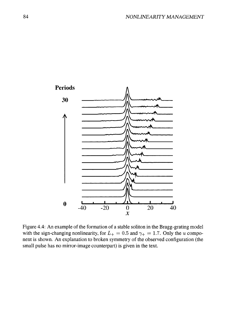
The formation of stable solitons in this system is accompanied by emission of radi-
ation, and, sometimes, by generation of a small additional pulse, as shown in Fig. 4.4.
The emission of radiation is conspicuous in the case when the stable soliton is close to
the lower stability border (in terms of
Fig.
4.3). On the other hand, in the unstable case
the initial pulse completely decays into radiation.
The stability diagram displayed in Fig. 4.3 was obtained from simulations of Eqs.
(4.8) and (4.9), starting from the initial configuration (1.33) with 9 = 0.484
•
IT,
which
4.3.
NONLINEARITYMANAGEMENT
83
Figure
4.3:
The stability diagram for the Bragg-grating solitons in the model with the
nonlinearity management, based on Eqs. (4.8), (4.9) and (4.11), (4.13). The stabil-
ity region is bounded by the lower solid curve, while the upper curve, the hyperbola
L+7+ = 1, is a border of the parametric area where the local Kerr coefficient period-
ically changes its sign. The dashed curve is the hyperbola L+j^ = 1/2 along which
the average value of nonlinearity is zero.
84
NONLINEARITY MANAGEMENT
Periods
30
Figure
4.4:
An example of the formation of
a
stable soliton in the Bragg-grating model
with the sign-changing nonlinearity, for L+ = 0.5 and
7-1-
= 1.7. Only the u compo-
nent is shown. An explanation to broken symmetry of the observed configuration (the
small pulse has no mirror-image counterpart) is given in the text.
4.3.
NONLINEARITYMANAGEMENT 85
is close to the stability-limiting value
6cr
~ 1.01
•
(7r/2) of the standard model (1.27),
(1.28) with constant coefficients. Additional simulations show that the stability region
has virtually no sensitivity to the variation of
^:
for example, decreasing 9 from 0.484-7r
to 0.452
• TT
(i.e., from arccos 0.05 to arccos
0.15;
recall the relation
u)
= cos
9
between
the frequency of the usual BG soliton (1.33) and 9) produces absolutely no detectable
change in the shape of the stability region.
4.3.4 Stability of solitons in the NLS equation with the periodic
nonlinearity management
For the sake of comparison of the manifestations of the NLM in different models, it is
relevant to generate a stability diagram for solitons in Eq. (4.15), with 7(2) taken again
as per Eqs. (4.11), (4.13). The simulations were run with the initial condition
uo{x) = 'risech{r]x), (4.16)
that would generate an exact soliton in the NLS equation with 7 = 1.
The result is that, for all the moderately narrow initial solitons (4.16), i.e., ones
with
T]
not too large, the respective stability diagram is almost indistinguishable from
its counterpart in Fig. 4.3. A difference between the BG and NLS models becomes
conspicuous if
r]
in the initial pulse (4.16) is high. One may expect that, for very
narrow solitons with large
r],
whose diffraction length ~ 1/77^ is much smaller than the
NLM period L = 1, the periodic change of the nonlinearity sign, as in Eq. (4.11), is
a very strong perturbation that may destroy the soliton (cf. the situation for the SSM
presented in the previous section, where solitons with the width ~
1
cannot exist in the
model with a very large modulation period L). Indeed, running the simulations of Eq.
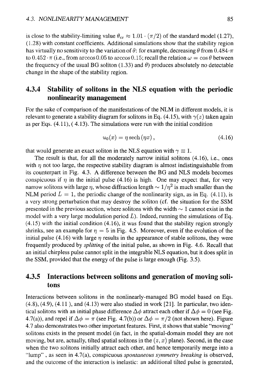
(4.15) with the initial condition (4.16), it was found that the stability region strongly
shrinks, see an example for r; = 5 in Fig. 4.5. Moreover, even if the evolution of the
initial pulse (4.16) with large
ry
results in the appearance of stable solitons, they were
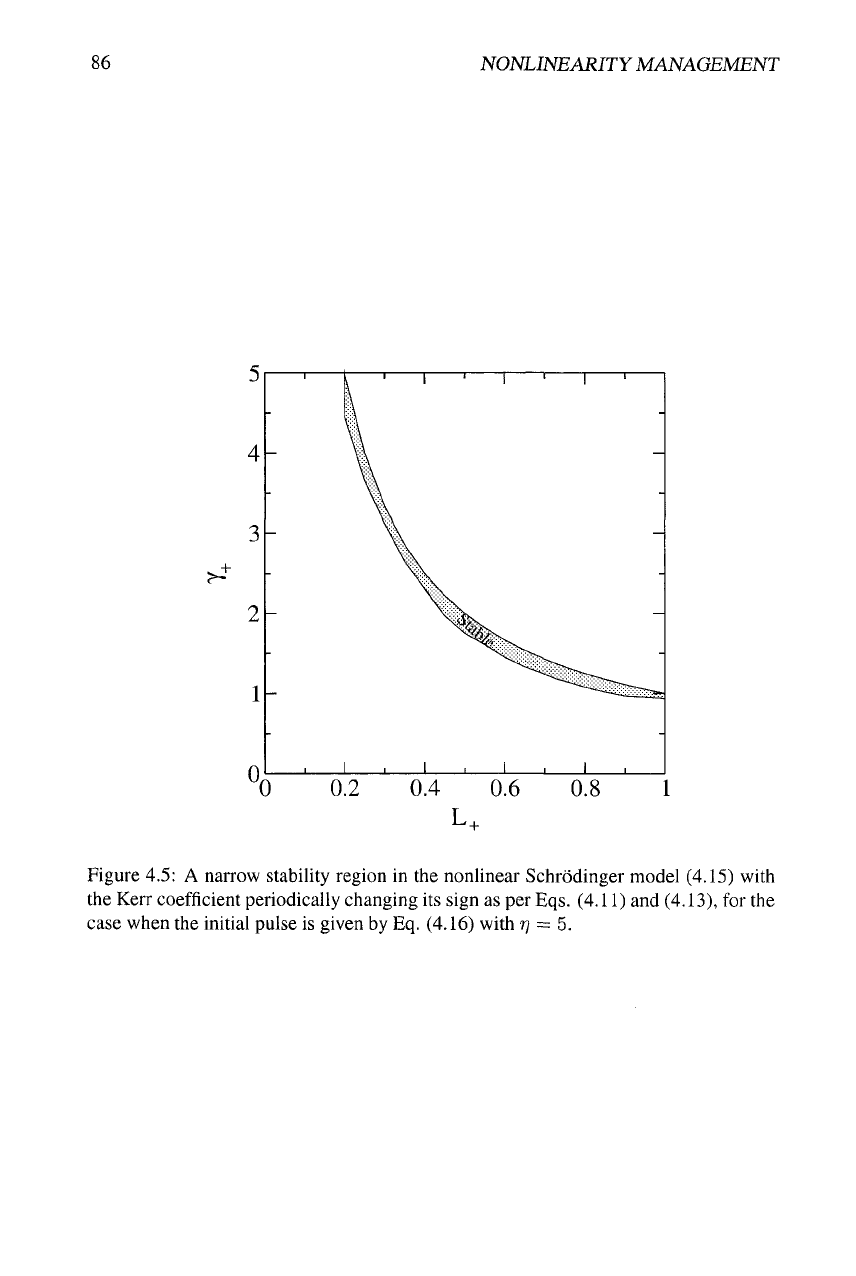
frequently produced by splitting of the initial pulse, as shown in Fig. 4.6. Recall that
an initial chirpless pulse cannot split in the integrable NLS equation, but it does split in
the SSM, provided that the energy of the pulse is large enough (Fig. 3.5).
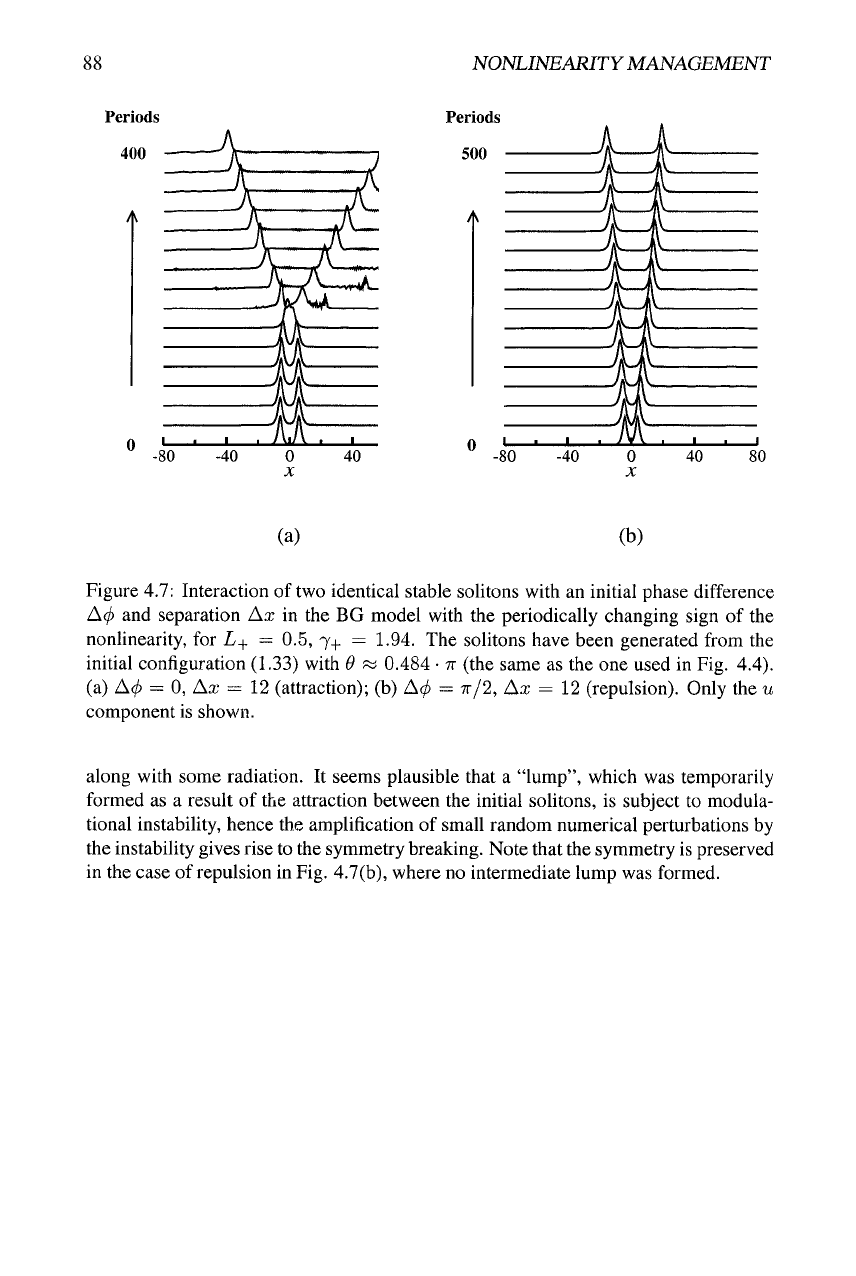
4.3.5 Interactions between soHtons and generation of moving soli-
tons
Interactions between solitons in the nonlinearly-managed BG model based on Eqs.
(4.8),
(4.9), (4.11), and (4.13) were also studied in work [21]. In particular, two iden-
tical solitons with an initial phase difference
Acj)
attract each other if A^ = 0 (see Fig.
4.7(a)), and repel if
Acj)
=
IT
(see Fig. 4.7(b)) or
A(f>
= 7r/2 (not shown here). Figure
4.7 also demonstrates two other important features. First, it shows that stable "moving"
solitons exists in the present model (in fact, in the spatial-domain model they are not
moving, but are, actually, tilted spatial solitons in the {z, x) plane). Second, in the case
when the two solitons initially attract each other, and hence temporarily merge into a
"lump"
, as seen in 4.7(a), conspicuous spontaneous symmetry breaking is observed,
and the outcome of the interaction is inelastic: an additional tilted pulse is generated,
86
NONLINEARITY MANAGEMENT
Figure 4.5: A narrow stability region in the nonlinear Schrodinger model (4.15) with
the Kerr coefficient periodically changing its sign as per Eqs. (4.11) and (4.13), for the
case when the initial pulse is given by Eq. (4.16) with
77
= 5.
4.3.
NONLINEARITY MANAGEMENT
87
Periods
200
,»V>**"'**'*
•—»»*
11
^'
iii4»»,>WliiWiii^|ll|f<>>»^i|ift¥<W^^
-40 -20 0 20 40
Figure
4.6:
An example of splitting of the narrow pulse (4.16) with
77
= 5 in the model
(4.15) into two secondary solitons with a smaller amplitude. The parameters of the
model are L+ = 0.35 and 7+ = 2.74. The propagation distance shown in this figure is
200 modulation periods.
88 NONLINEARITY MANAGEMENT
Periods
500 •
-80 -40
0
X
40 80
(a)
(b)
Figure 4.7: Interaction of two identical stable solitons with an initial phase difference
A^ and separation Ax in the BG model with the periodically changing sign of the
nonlinearity, for L+ = 0.5, 7+ = 1.94. The solitons have been generated from the
initial configuration (1.33) with 9 w 0.484
•
n (the same as the one used in Fig. 4.4).
(a)
A<f)
= 0, Ax = 12 (attraction); (b) A(f) =
TT/2,
AX = 12 (repulsion). Only the u
component is shown.
along with some radiation. It seems plausible that a "lump", which was temporarily
formed as a result of the attraction between the initial solitons, is subject to modula-
tional instability, hence the amplification of small random numerical perturbations by
the instability gives rise to the symmetry breaking. Note that the symmetry is preserved
in the case of repulsion in Fig. 4.7(b), where no intermediate lump was formed.
Chapter 5
Resonant management of
one-dimensional solitons in
Bose-Einstein condensates
It was explained in the Introduction that the technique based on the Feshbach resonance
(FR),
which makes it possible to control the size and sign of the scattering length of
atomic collisions in BEC, i.e., the coefficient in front of the cubic term in the corre-
sponding GPE (Gross-Pitaevskii equation), has become a very important tool in the
experiment [81, 148, 157], and also is a strong incentive for the development of the-
oretical analysis. Especially interesting is the possibility to control the nonlinearity
coefficient by ac (time-periodic) magnetic field, which brings the nonlinearity manage-
ment concept into the realm of
BEC.
In the ID setting, this technique was developed
under the name of the Feshbach-resonance management (FRM) in work [90]. The
analysis was focused not on solitons proper, but rather on more general states whose
localization was supported by the external parabolic trapping field (in the experiment,
magnetic or optical trap is always necessary [141]). Additionally, the resonant action
of the harmonic time modulation of the nonlinearity coefficient on fundamental and
higher-order solitons in the NLS equation without external potential was recently stud-
ied in work
[153].
Main results obtained for the FRM-driven localized nonsoliton and
soliton states in the ID setting are summarized in this chapter.
5.1 Periodic nonlinearity management in the one-dimensional
Gross-Pitaevskii equation
It is known that the 3D Gross-Pitaevskii equation (GPE) (1.39) for BEC tightly con-
fined in two transverse directions {x and y), and loosely confined by the parabolic
potential fl'^x'^/2 along the longitudinal axis x, can be reduced, by averaging in the