Malomed B.A. Soliton Management in Periodic Systems
Подождите немного. Документ загружается.

110 WAVEGUIDING-ANTIWAVEGUIDING SYSTEM
where
T
is the trace of the matrix,
T = 2cos (a;+L+) cosh (w_L_) + (w?.
—
w^) (w-).w_)~ sin (a;+L+) sinh (w_L_) .
(6.16)
As it follows fromEqs. (6.15) and (6.16), the stability conditions |/Ui,2| = 1 are met if
\T\
< 2, or, in an explicit form,
cos
{uj+L+)
cosh (a;_L_) sin (a;+L+) sinh (a;_L_)
<1.
(6.17)
This inequality represents the full stability region in an explicit form, as predicted by
the analytical approximation. Note that the condition (6.17) is trivially satisfied in the
case of the uniform WG, L_ = 0, and it is definitely not satisfied in the opposite case
of the uniform AWG, L+ = 0.
It is easy to find a minimum value {L+)^^^ of the WG segment which is necessary
to achieve the stabilization at given values of the parameters L_ and
ui±:
as it follows
fromEq. (6.17),
'^+ (-^+)min = arCCOS
/cosh^ {u-L-) + a^ sinh^ (a;_L_
—
arctan(Qtanh(w_L_)), (6.18)
where ft = (w^ - w?.) / {2UJ+UJ^). It is easy to show that the expression (6.18) is
always positive. Note that it remains finite in the limit of L_ -^ oo, which is ex-
plained by a possibility to find a special value of the parameter
u:+L+
such that a WG
segment inserted between two AWG segments mixes the eigenmodes so that the one
corresponding to the unstable eigenvalue -f-w- in the AWG section preceding the WG
one will go over into an eigenmode corresponding to the stable eigenvalue —w_ in the
next AWG section. In fact, the mixing of the stable and unstable AWG eigenmodes by
the WG segments is a mechanism which makes the stable channeling of the beam in
the alternate structure possible.
A noteworthy property of the stability condition (6.17) is that the stabilization of
the trapped beam does not monotonically enhance with the increase of the duty-cycle
ratio L+/L- of the WG and AWG segments. For instance, in the case of w^ = uit the
inequality (6.17) takes the form |cos (a;+L+)| < sech {uj-L-). If one increases L4.,
keeping L_ fixed, the latter condition is met in intervals
arccos [sech (a;_L_)] + 27rn < w+L+ <
—
arccos [sech (a;_L_)] + 27r (n + 1),
(6.19)
n = 0,1,2,..., and it is not met in gaps between the intervals. An implication of this
is that, even if the length of the AWG segment is very small, there are some values
of the ratio L+/L-, which may be arbitrarily large, around which the trapped beam is
unstable. The non-monotonic dependence of the stability on the duty cycle is confirmed
by numerical results displayed in the following section.
6.4. NUMERICAL RESULTS
111
!
•- 4
i
1
i
i
t
T
i
It
11
ll
!
—
(a)
(b)
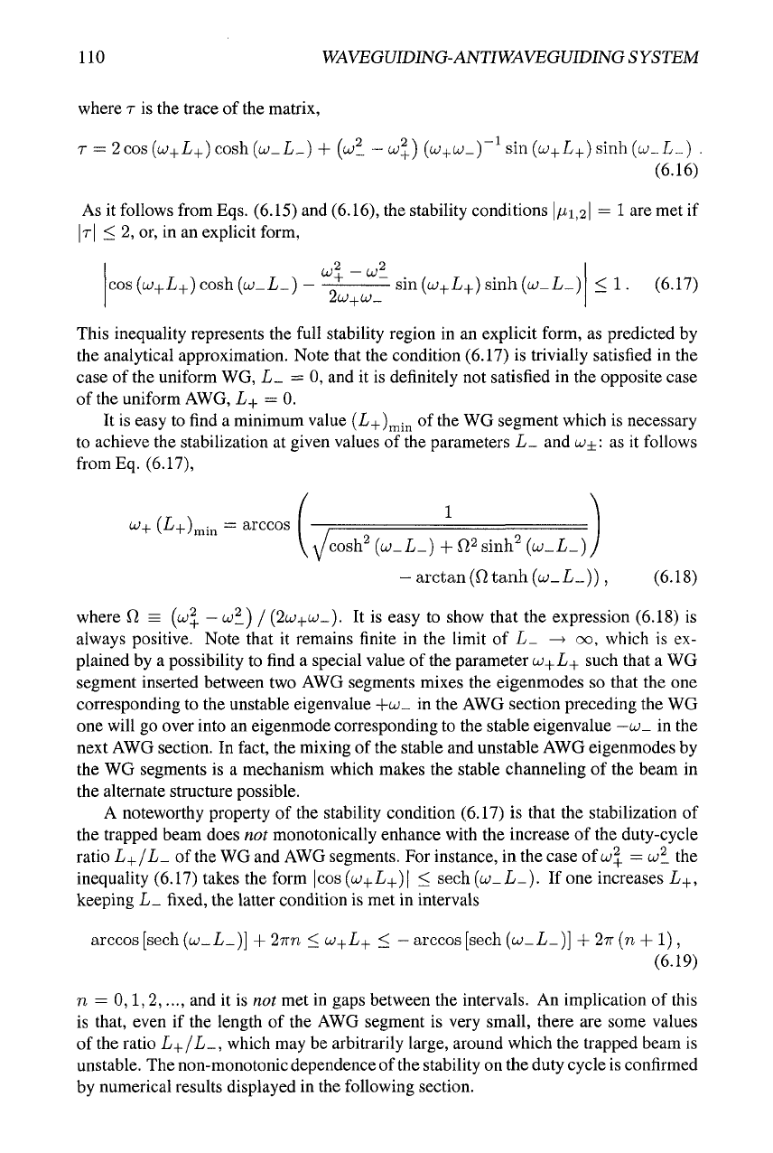
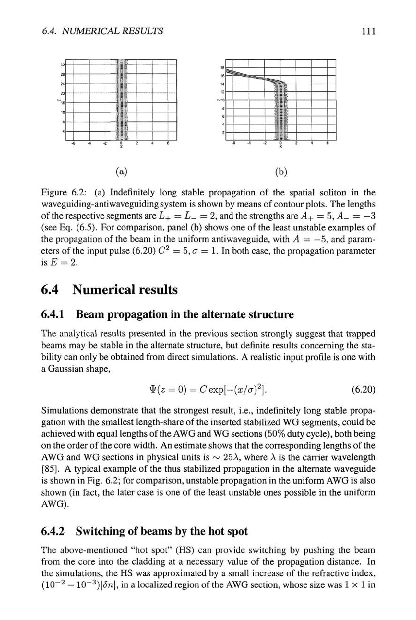
Figure 6.2: (a) Indefinitely long stable propagation of the spatial soliton in the
waveguiding-antiwaveguiding system is shown by means of contour
plots.
The lengths
of the respective segments are L+ = L_ = 2, and the strengths are ^+ = 5, A- = —3
(see Eq. (6.5). For comparison, panel (b) shows one of the least unstable examples of
the propagation of the beam in the uniform antiwaveguide, with A = ~5, and param-
eters of the input pulse (6.20) C^ = 5,
CT
= 1. In both case, the propagation parameter
is £: = 2.
6.4 Numerical results
6.4.1 Beam propagation in tiie alternate structure
The analytical results presented in the previous section strongly suggest that trapped
beams may be stable in the alternate structure, but definite results concerning the sta-
bility can only be obtained from direct simulations. A realistic input profile is one with
a Gaussian shape,
*(z = 0) = Cexp[-(x/<7)2].
(6.20)
Simulations demonstrate that the strongest result, i.e., indefinitely long stable propa-
gation with the smallest length-share of the inserted stabilized WG segments, could be
achieved with equal lengths of
the
AWG and WG sections (50% duty cycle), both being
on the order of the core width. An estimate shows that the corresponding lengths of the
AWG and WG sections in physical units is ~ 25A, where
A
is the carrier wavelength
[85].
A typical example of the thus stabilized propagation in the alternate waveguide
is shown in Fig. 6.2; for comparison, unstable propagation in the uniform AWG is also
shown (in fact, the later case is one of the least unstable ones possible in the uniform
AWG).
6.4.2 Switching of beams by the hot spot
The above-mentioned "hot spot" (HS) can provide switching by pushing the beam
from the core into the cladding at a necessary value of the propagation distance. In
the simulations, the HS was approximated by a small increase of the refractive index,
(10~^
—
10"'^)
15n|,
in a localized region of the AWG section, whose size was 1 x 1 in
112 WAVEGUIDING-ANTIWAVEGUIDING SYSTEM
the normalized units, and Sn is the same as in
Eq.
(6.3). The HS strength corresponding
to these values of the parameters is sufficient to control the switching; in real-world
units,
this implies that the net power of
the
beam creating the HS should be between 1%
and
0.1%
of the signal-beam's power (this power, although small, is much higher than
the fluctuation level, i.e., random fluctuations cannot switch the beam accidentally).
Detailed simulations demonstrate that a virtually identical switching effect is produced
by various particular forms of
the
distribution of
the
refractive-index perturbation inside
the HS, provided that the net perturbation, integrated over the HS, is fixed.
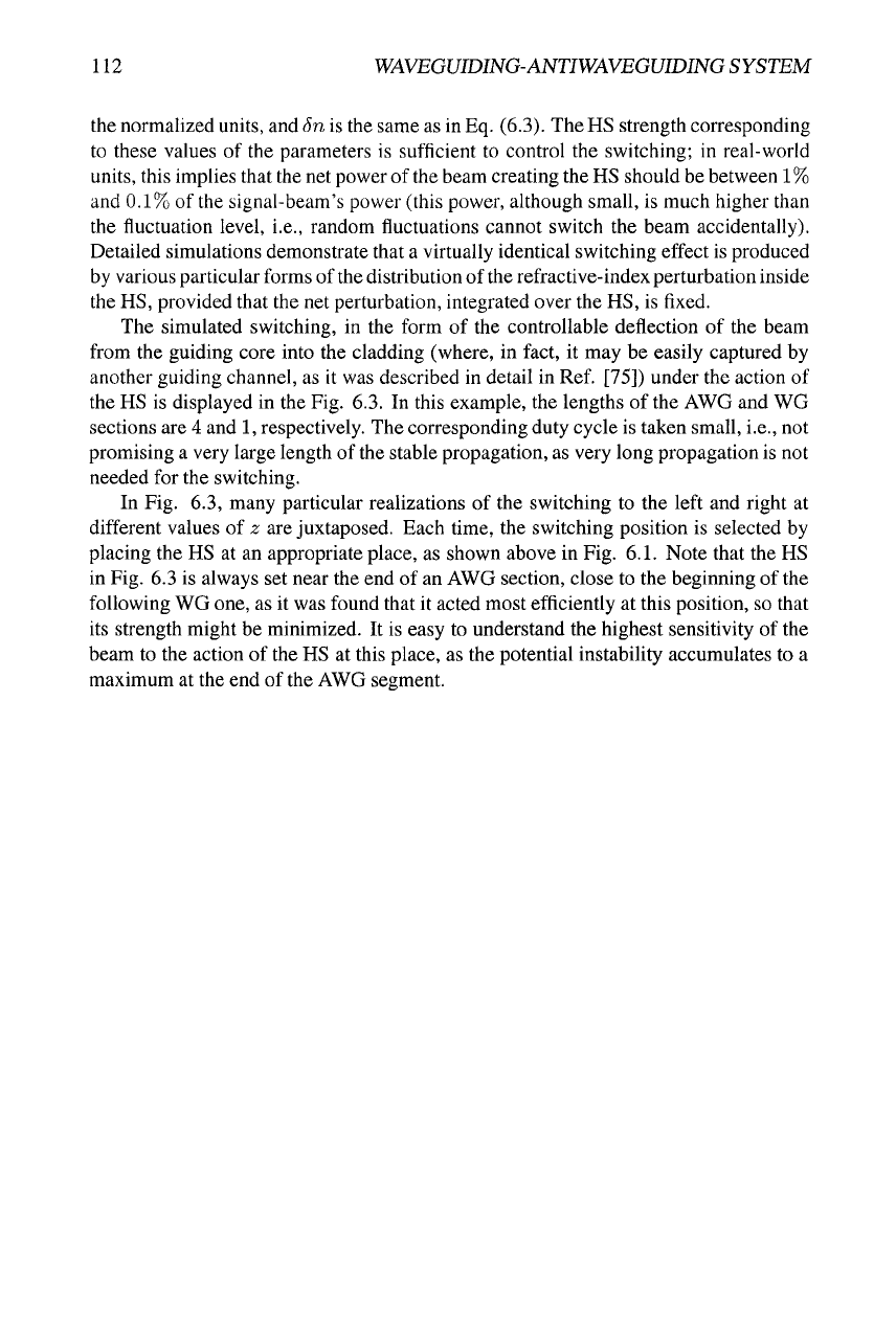
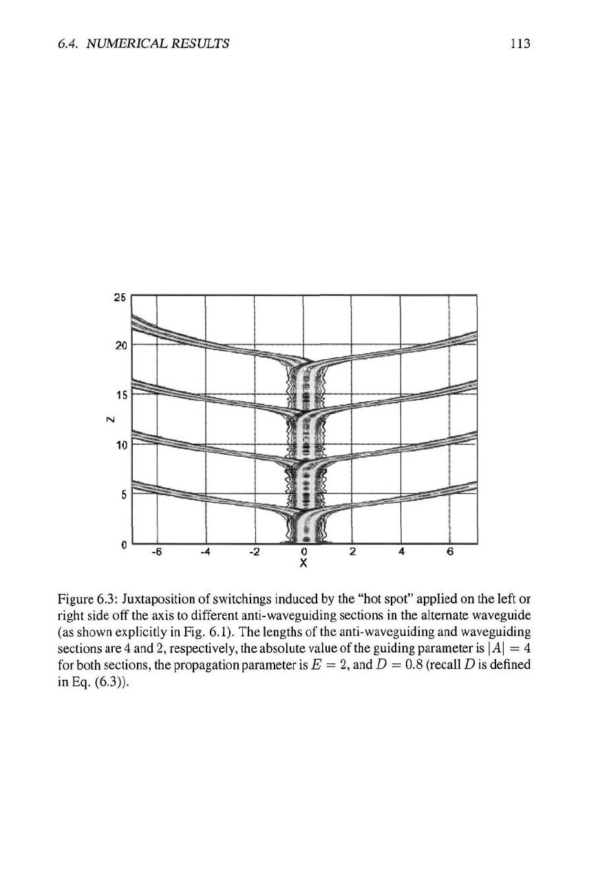
The simulated switching, in the form of the controllable deflection of the beam
from the guiding core into the cladding (where, in fact, it may be easily captured by
another guiding channel, as it was described in detail in Ref. [75]) under the action of
the HS is displayed in the Fig. 6.3. In this example, the lengths of the AWG and WG
sections are 4 and 1, respectively. The corresponding duty cycle is taken small, i.e., not
promising a very large length of the stable propagation, as very long propagation is not
needed for the switching.
In Fig. 6.3, many particular realizations of the switching to the left and right at
different values of z are juxtaposed. Each time, the switching position is selected by
placing the HS at an appropriate place, as shown above in Fig. 6.1. Note that the HS
in Fig. 6.3 is always set near the end of an AWG section, close to the beginning of the
following WG one, as it was found that it acted most efficiently at this position, so that
its strength might be minimized. It is easy to understand the highest sensitivity of the
beam to the action of the HS at this place, as the potential instability accumulates to a
maximum at the end of the AWG segment.
6.4. NUMERICAL RESULTS 113
Figure
6.3:
Juxtaposition of switchings induced by the "hot spot" applied on the left or
right side off the axis to different anti-waveguiding sections in the alternate waveguide
(as shown explicitly in Fig. 6.1). The lengths of the anti-waveguiding and waveguiding
sectionsare4and2, respectively, the absolute value of the guiding parameter is \A\ = 4
for both sections, the propagation parameter
is
£^ = 2, and D = 0.8 (recall D is defined
inEq. (6.3)).
Chapter 7
Stabilization of spatial solitons
in bulk Kerr media with
alternating nonlinearity
7.1 The model
The usual
(2+
l)-dimensional
NLS
equation governing the spatial evolution of light sig-
nals in bulk (3D) optical media with the
x*^^^
(Kerr) nonlinearity cannot support stable
spatial solitons in the form of cylindrical beams: if the nonlinearity is self-defocusing
(negative), any beam spreads out, while in the case of the self-focusing (positive) non-
linearity, a stationary-beam solution with a critical value of its norm (integral power)
does exist, as was demonstrated by Chiao, Garmire, and Townes in 1964 (as a mat-
ter of fact, it was the first example of a soliton considered in nonlinear optics, and is
frequently referred to as a
Townes
soliton, TS), but it is (weakly) unstable because of
the possibility of the weak collapse in the 2D NLS equation [29, 159]. In work [30],
it was shown, by means of direct simulations, that the beam can be pardy stabilized if
the nonlinearity coefficient in the 2D NLS equation is subjected to weak spatial mod-
ulation along the propagation direction, so that the beam's power (which is virtually
constant, as radiative losses turn out to be negligible) effectively oscillates about the
accordingly modulated critical value, being sometimes slightly above and sometimes
slightly below it. As a result, it was observed that the beam could survive over a large
propagation distance, although eventually is was destroyed by the instability.
A model of a strong NLM (nonlinearity management) for the bulk medium, with
the periodic alternation of the sign of the local Kerr coefficient (the same as in the ID
NLM model in Eq. (4.II)), was proposed in paper
[165]:
iu^ + -\7lu +
-f{z)\u\\
= 0, (7.1)
116 SPATIAL SOLITONS IN BULK MEDIA
7(.) = |^+' ., if 0<^<^+' (7.2)
'^ ' \ 7_, if L+< z < L++L-, ^ ^
where the diffraction operator Vj^ acts on the transverse coordinates x and y. The
main result of work [165] is that this model provides for complete stabilization of the
(2+l)-dimensional solitons, as shown in detail below. The consideration of this model
was not only interesting in its own right, but also served as a pattern for prediction of
the stabilization of 2D BECs under the action of the time-periodic FRM, see the next
chapter.
Axisymmetric spatial solitons, as solutions to Eq. (7.1), are sought for in the form
u{z, r, 9) = exp{iS9)U{z, r), (7.3)
where r and 6 are the polar coordinates in the (x, y) plane, S is an integer vorticity
("spin"), and the function t/(z, r) obeys the equation
1 / 1 _ ^
2 V r r-^
iU, + -[ Urr +zUr-^U)+ J{z)\U\^'U = 0. (7.4)
7.2 Variational approximation
First of all, VA may be applied to Eq. (7.4). To this end, the following ansatz is
adopted,
U = A{z)r'^ exp [ih{z)r'^ +
i(t){z)]
sech ( -^ j , (7.5)
where A, b and a are the soliton's amplitude, chirp and width, and
(p
is the phase, cf.
the ID ansatz (2.6). An essential difference in the 2D case is the necessity to add the
multipliers r^, for the case of S j^ 0 (by definition, S is positive). Then, the following
set of the variational equations for the parameters of the ansatz (7.5) can be derived.
First, due to the conservation of energy, there is a dynamical invariant
which makes it possible to eliminate the amplitude A from the equations. After that,
the VA reduces to a second-order equation for a{z),
dz^ ^
AS) r{S)
AS) AS) 'y^f
the chirp being expressed as b{z) = {2a)~^da/dz, cf. similar variational equations
(S)
(2.12) and (2.11) for the ID soliton. Numerical constants /^ 24 ai'e integrals resulting
from VA; for 5
==
0 (zero-spin beam), they are l[°l^ w (1.352,0.398,0.295).
In the NLM model with the periodic modulation (7.2), equation (7.7) can be solved
inside each interval where 7 is constant. The result is
^] +r = HV, (7.8)
1.2. VARIATIONAL APPROXIMATION 117
where V = a?, H (which is actually the Hamiltonian of
Eq.
(7.7) with 7 = const) is
an arbitrary integration constant, and
r.sLAj:.
(7.9)
-'1
Within the interval 0 < z < L+, the parameter F keeps a constant value r+,
then it assumes another constant value r_ in the interval L^ < z < L+ + L-, and
this configuration repeats itself periodically. The formulas can be additionally rescaled
to set L_ = 1 and r_ = 1, leaving one with two irreducible control parameters,
L+ = L and r+ = F (note that the definition of F implies that, once it was set
r_ = 1, then F = F_|_ may only take values smaller than 1, including negative values).
Across each junction point where 7 flips its sign, the values of V and dV/dz are related
according to the physical conditions that the width and chirp of the pulse, as functions
of z, must be continuous. As immediately follows from the above equations, this
simply means that both V and dV/dz are continuous across the
jump.
Such boundary
conditions are essentially easier to handle than their counterparts in the case of DM,
where the continuity of the chirp, given by the expression b = —2/3{z)a{da/dz) (see
Eq. (2.11)), and the jump of the GVD coefficient f3{z) at the junction point imposes a
jump condition on the derivative da/dz. The simplification of the boundary conditions
in the present NLM model makes it possible to obtain results in a completely analytical
form, as shown below (which was impossible in the DM model).
Starting with arbitrary initial values
VQ
and
VQ
of V{z) and dV/dz at 2 = 0, one
can derive a map that yields the values
VQ
and
VQ
of the same variables at the end of
the period, i.e., at z
—
L+ + L^ = I + L. Straightforward integration of
Eq.
(7.8) in
the segments L±, with regard to the continuity of V and dV/dz at the junction points,
makes it possible to derive the map in an explicit although rather cumbersome form.
Nevertheless, a fixed point (FP) of the map, which corresponds to the quasi-stationary
propagation of the beam, can be found in a simple form:
This FP exists only for negative values of the coefficient (7.9), F < —1/L.
Calculating the path-average value of the nonlinearity coefficient, with regard to
the normalizations adopted here,
_ _ L+7+ + L-7- _ 8/2 (L + 1) - /iF, (LF + 1)
^" L+ + L_ 8/4 (L + 1) ' ^ '
it is easy to see that FPs (7.10) may only exist with positive 7 (corresponding to
self-
focusing on average). Taking into account the above-mentioned necessary condition
r < —1/L and normalizations, Eq. (7.11) predicts the minimum value of the path-
average nonlinearity coefficient at which the FPs exist: (7)jnin = -^2 /M ~ 1-3453.
This result is quite natural, as it would be strange to expect the existence of quasi-
stationary soliton beams in the case when the average nonlinearity is self-defocusing
on average. On the other hand, it is relevant to recall that ID stable solitons do exist in
118
SPATIAL SOLITONS IN BULK MEDIA
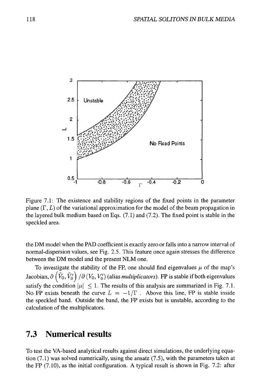
Figure 7.1: The existence and stability regions of the fixed points in the parameter
plane (F, L) of the variational approximation for the model of the beam propagation in
the layered bulk medium based on Eqs. (7.1) and (7.2). The fixed point is stable in the
speckled area.
the DM model when the PAD coefficient is exactly zero or falls into a narrow interval of
normal-dispersion values, see Fig. 2.5. This feature once again stresses the difference
between the DM model and the present NLM one.
To investigate the stability of the FP, one should find eigenvalues /i of the map's
Jacobian, 9 (Vij), V'o) /^ (^o,
VQ)
(alias multiplicators). FP is stable if both eigenvalues
satisfy the condition |/i| < 1. The results of this analysis are summarized in Fig. 7.1.
No FP exists beneath the curve L =
—
1/r . Above this line, FP is stable inside
the speckled band. Outside the band, the FP exists but is unstable, according to the
calculation of the multiplicators.
7.3 Numerical results
To test the VA-based analytical results against direct simulations, the underlying equa-
tion (7.1) was solved numerically, using the ansatz (7.5), with the parameters taken at
the FP (7.10), as the initial configuration. A typical result is shown in Fig. 7.2: after
1.3. NUMERICAL RESULTS 119
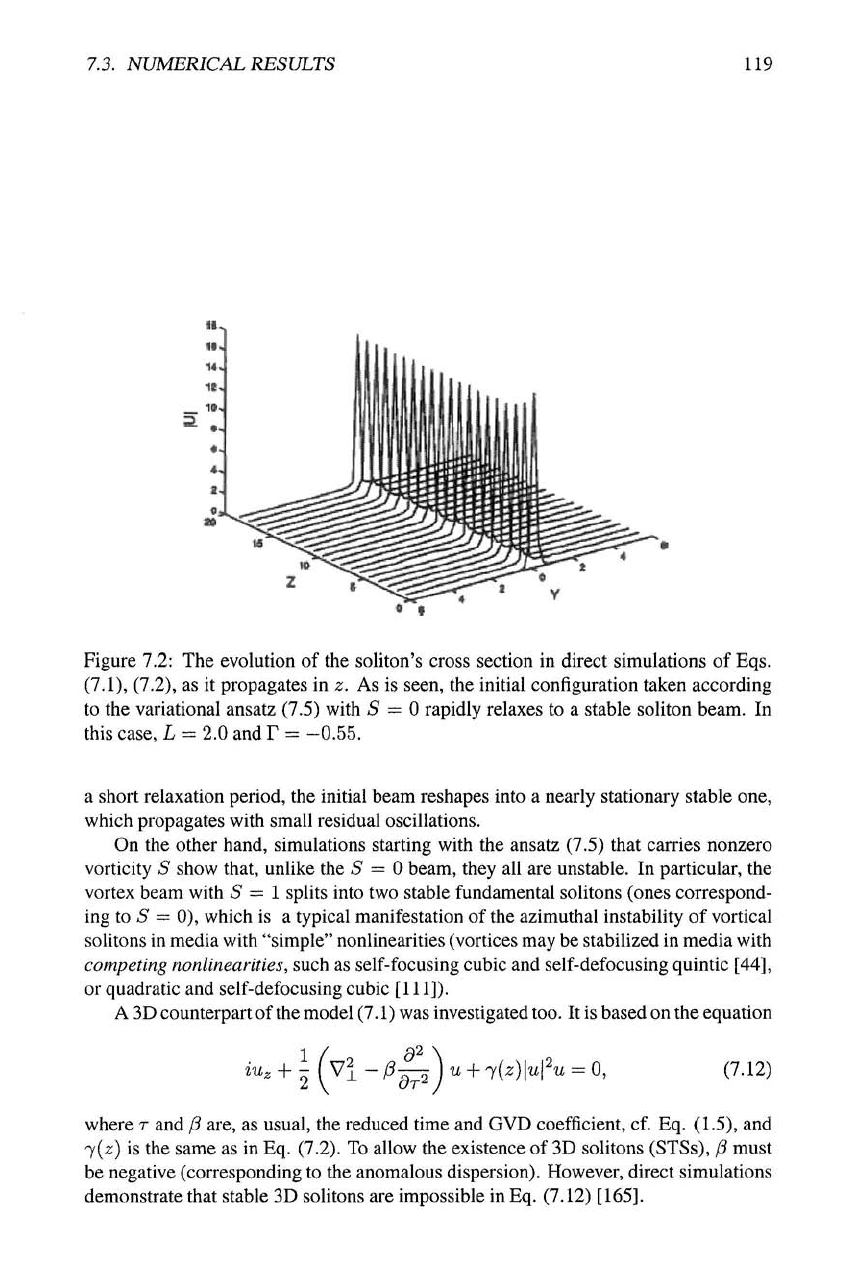
Figure 7.2: The evolution of the soliton's cross section in direct simulations of Eqs.
(7.1),
(7.2), as it propagates in z. As is seen, the initial configuration taken according
to the variational ansatz (7.5) with 5 = 0 rapidly relaxes to a stable soliton beam. In
this case, L = 2.0 and T =
-0.55.
a short relaxation period, the initial beam reshapes into a nearly stationary stable one,
which propagates with small residual oscillations.
On the other hand, simulations starting with the ansatz (7.5) that carries nonzero
vorticity S show that, unlike the 5 = 0 beam, they all are unstable. In particular, the
vortex beam with 5=1 splits into two stable fundamental solitons (ones correspond-
ing to 5 = 0), which is a typical manifestation of the azimuthal instability of vortical
solitons in media with "simple" nonlinearities (vortices may be stabilized in media with
competing nonlinearities, such as self-focusing cubic and self-defocusing quintic [44],
or quadratic and self-defocusing cubic [111]).
A 3D counterpart of
the
model (7.1) was investigated
too.
It is based on the equation
-U-i^"^
.
+ 'y(z)\u\\ = 0,
(7.12)
where T and
/3
are, as usual, the reduced time and GVD coefficient, cf. Eq. (1.5), and
7(z) is the same as in Eq. (7.2). To allow the existence of 3D solitons (STSs),
(3
must
be negative (corresponding to the anomalous dispersion). However, direct simulations
demonstrate that stable 3D solitons are impossible in Eq. (7.12)
[165].
Chapter 8
Stabilization of two-dimensional
solitons in Bose-Einstein
condensates under
Feshbach-resonance
management
The possibility to stabilize (2+l)-dimensional spatial solitons by means of the peri-
odic alternation of the sign of the Kerr coefficient in a layered bulk material suggest a
physically different but mathematically similar possibility to stabilize 2D soliton-like
BEC configurations by means of the ac-FRM technique, which amount to making the
nonlinearity coefficient in the corresponding 2D Gross-Pitaevskii equation (GPE) a si-
nusoidal function of time. This possibility was first independently explored in works
[5] and
[150].
Additional results, including the case of a 3D condensate strongly con-
fined in one direction, which makes it nearly two-dimensional, were reported in paper
[130],
and a similar mechanism providing for stabilization of a two-component 2D
soliton in a system of
two
nonlinearity coupled GPEs was investigated too
[128].
Here,
main results for this important problem will be presented, chiefly following paper [5].
It will also be shown that the ac-FRM technique (if acting alone) cannot stabilize 3D
solitons.