Malomed B.A. Soliton Management in Periodic Systems

Подождите немного. Документ загружается.

132 MULTIDIMENSIONAL DISPERSION MANAGEMENT

ficients is denoted here as —D, instead of

/?.

It is subject to the same DM modulation

asinEq. (1.49),

^^^' \ D^<0,L+<z<L+ + L^=L, ^^-^^

which repeats itself periodically with the period L (in terms of D, the anomalous and

normal GVD correspond, respectively, to D > 0 and D < 0). Note that Eq. (9.1))

has a manifest property of the Galilean invariance: if uo(x, z, r) is a solution, a two-

parametric family of "boosted" (moving) solutions can be generated from it as follows:

U{X,Z,T)

— exp i{qx

— (jjT

q^z

—

-uP' D{z)dz

—

qz,z,T +

/ D{z)dz

, (9.3)

where q and w are two arbitrary real parameters ("Galilean boosts"), which is to be

compared with the similar invariance of the ID NLS equation, see Eq. (1.6).

To cast the model into a normalized form, one can set, by means of obvious rescal-

ings,

D+ = 1, L = 2. The ratio L-/L+ remains an irreducible parameter, but it is

well known that, in the usual DM model for optical fibers, the results do not depend

on this ratio, nor separately on the soliton's temporal width Tpwuu, but rather on the

DM strength, S = {D+L+ + \D^\L^) /T|WHM' see Eq. (2.25). Therefore, it will

be fixed here that L+ = L_ = 1. Then, in addition to S, the only remaining free

parameter of the model is the PAD (path-average dispersion), which takes the form

I5.5±i±±i^ = la

Z,_),

,9.4)

with regard to the normalizations D+ = \,L± = 1. The remaining parameter Z?_ can

be expressed in terms of D: as it follows from Eq. (9.4), D_ = 2D

—

It is relevant to mention that this 2D model is somewhat similar to another one,

that was recently introduced in work [2]; it differs by sinusoidal modulation of D{z),

instead of the piece-wise constant DM map adopted in Eq. (9.2), and, most impor-

tantly, by the fact that (in the present notation) it has the same modulated coefficient

multiplying both the GVD term

UTT

and the diffraction one,

u^x'-

iu^

+ -[Do + Di sin {kz)] {u^x + UTT) + \u\^u = 0, (9.5)

with Do > 0. In fact, this model was motivated by a continuum limit of some discrete

systems; as concerns the context of nonlinear optics, it would be difficult to introduce

the periodic reversal of the sign of the transverse diffraction (the coefficient in front of

Uxx)-

There is a great difference between Eq. (9.1), which is strongly anisotropic in

the plane {x, r), and the isotropic equation (9.5).

9.2 Variational approximation

The VA (variational approximation) is a natural tool for the analysis of solitons in Eq.

(9.1).

To apply it, a straightforward Gaussian ansatz is adopted (cf. ansatze (2.6) and

9.2. VARIATIONAL APPROXIMATION

133

(8.5)),

u = A{z) exp

ifpiz)

—

W^lyz)

T^{z)

+ ' [b{z)x^+p{z)'

(9.6)

where A and

(f)

are the amplitude and phase of the soliton, W and T are its transverse

and temporal widths (the latter is related to the above-mentioned full-width-at-half-

maximum as follows: TpwHM = 2^/ln2T), and b and

are the spatial and temporal

chirps. The Lagrangian from which the 2D version of

Eq.

(9.2) is derived is

-l-oo

{uzU*

~ ulu)

—

\ux\

—

D{z)\ur\ +

\u\'^

dxdr. (9.7)

Substitution of the ansatz (9.6) into the Lagrangian yields an effective Lagrangian,

-LefF = A^WT[4:(j)'-b'W'^-l3'T^~W-'^-DT

2rp21

+A'

- h'W -

D{z)f3'T'\

(9.8)

where the prime stands for d/dz.

The variational equation 5L/5(j) = 0, applied to the expression (9.8), yields, as

always, the energy-conservation relation, dE/dz = 0, where

E = A^WT.

Equation (9.9) is used to eliminate A? from subsequent equations. Then, the term'

in the Lagrangian may be dropped, and it takes the form

(9.9)

4L,

eff

•KE

h'W'^ -

/3'T'^

D{zl

]y2 J'2

-yW^-D{z)(i^T\ (9.10)

Varying the latter expression with respect to W, T and

yields the following Euler-

Lagrange equations:

__W' __ T

^^W^^^(z)f'

(9.11)

W^ 2W^T'

f^ ~ 2WT'^ '

(9.12)

(9.13)

Note that, as is known from the variational approach to the description of collapse

in the 2D NLS equation [48], in the case of

= const < 0, fixed-point (FP) solutions

to the VA equations (9.12) and (9.13) are degenerate: the FP exists at a single value

of the energy, E = 2\/D, and, at this special value of E, there is a family of FPs

with T = \/DW (W is arbitrary). These results exactly correspond to the existence

of the TS (Townes soliton) in the isotropic 2D NLS equation. The family of the TS

134 MULTIDIMENSIONAL DISPERSION MANAGEMENT

solutions are found at a single value of the energy, but with arbitrary width. Within the

framework of Eqs. (9.12) and (9.13), all the FPs corresponding to

— const

> 0

are weakly unstable (against small perturbations that grow with

linearly, rather than

exponentially, which corresponds to the fact that the collapse is weak in the 2D case,

on the contrary to strong collapse in three dimensions).

In the case of the piece-wise constant modulation corresponding to Eq. (9.2), the

variables W,

W, T

and /3 at junctions between the segments with D

D± must be

continuous. As it follows from Eq. (9.11), the continuity of the temporal chirp I3{z)

implies

jump of T' when passing from D_ to D+, or vice versa:

{T')D=D,=^_{T')„^^_^.

(9.14)

9.3 Numerical results

Both the variational equations (9.12), (9.13) and the underlying GPE (9.1) were simu-

lated numerically. In the latter case, the initial state was taken as per the ansatz (9.6),

with zero spatial chirp (obviously, a point at which it vanishes can always be found, so

this choice does not imply any special restriction), while the initial temporal chirp, /3o,

was included:

AQ exp

\{wS

^ei-'^'^'

(9.15)

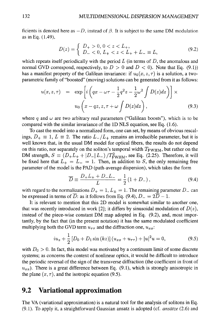
Completely stable periodically oscillating solitons were easily found in direct PDE

simulations, closely following the prediction provided by the VA. As a typical exam-

ple,

Fig. 9.1 shows a sequence of the soliton's snapshots through one (40th) cycle of

the evolution. This picture remains identically the same, for instance, at the 80th cy-

cle,

attesting to the true stability of the solitons in the 2D DM model. No leakage (net

radiation loss) from the established soliton was observed, up to the accuracy of numer-

ical simulations. This implies that a small amount of radiation, emitted from the pulse

when it passes the normal-dispersion slice, is absorbed back into it in the slice with

anomalous dispersion.

The shape of the pulse in Fig. 9.1 remains very close to a Gaussian, which explains

why the VA provides for good accuracy in this case. The evolution of the temporal

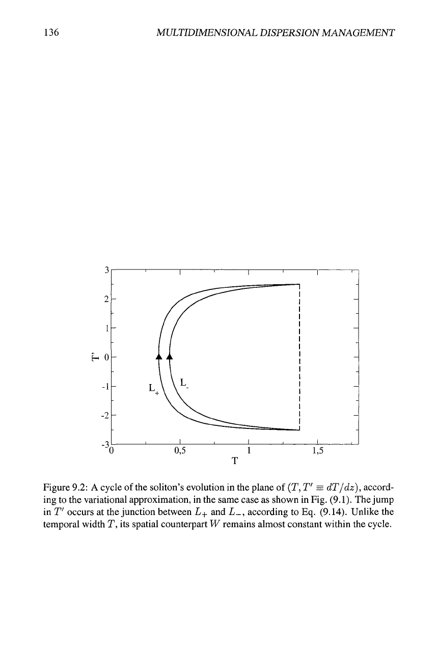
width T{z) for the same parameters, as predicted by the VA, is displayed in Fig. 9.2.

On the contrary to T{z), the spatial width W{z) remains nearly constant, suggesting

that the stable 2D soliton may be realized, in loose terms, as a "product" of

the

temporal

DM soliton in the r-direction, and ordinary spatial soliton localized in

(a factorized

ansatz of this type was proposed for the consideration of multidimensional optical soli-

tons in work [97]). Comparison shows that the PDE numerical solution indeed agrees

well with the VA prediction.

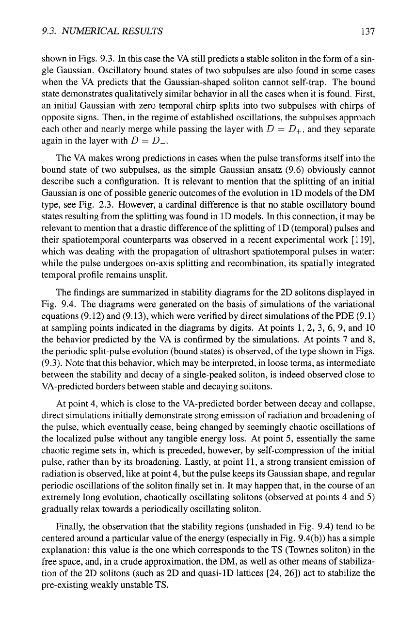
However, in some other cases direct simulations of Eq. (9.1) reveal periodic evo-

lution in a drastically different form: the initial pulse splits into two subpulses, which

do not fully separate, but rather form an oscillatory bound state, examples of which are

9.3.

NUMERICAL RESULTS

135

1/4 cycle

Figure

9.1:

Evolution of

the

intensity distribution in a stable 2D soliton through a cycle

of its propagation in the dispersion-managed nonlinear planar waveguide, described by

Eqs.

(9.1) and (9.2), with D+ = -£>_ = 1, L+ = L_ = 1. Parameters of the initial

pulse (9.15) are To = 1.35,

= 1.35, E = 1, and

/?o

-1.85.

Snapshots are taken

at points corresponding to the start,

1/4,1/2

and 3/4 of the cycle.

136

MULTIDIMENSIONAL DISPERSION MANAGEMENT

H 0

Figure 9.2: A cycle of the soliton's evolution in the plane of (T, T' = dT/dz), accord-

ing to the variational approximation, in the same case as shown in Fig. (9.1). The jump

in T' occurs at the junction between L+ and L_, according to Eq. (9.14). Unlike the

temporal width T, its spatial counterpart W remains almost constant within the cycle.

9.3.

NUMERICAL RESULTS 137

shown in

Figs.

9.3. In this case the VA still predicts a stable soliton in the form of

sin-

gle Gaussian. Oscillatory bound states of two subpulses are also found in some cases

when the VA predicts that the Gaussian-shaped soliton cannot self-trap. The bound

state demonstrates qualitatively similar behavior in all the cases when it is found. First,

an initial Gaussian with zero temporal chirp splits into two subpulses with chirps of

opposite signs. Then, in the regime of established oscillations, the subpulses approach

each other and nearly merge while passing the layer with D = D+, and they separate

again in the layer with D = Z)_.

The VA makes wrong predictions in cases when the pulse transforms itself into the

bound state of two subpulses, as the simple Gaussian ansatz (9.6) obviously cannot

describe such a configuration. It is relevant to mention that the splitting of an initial

Gaussian is one of possible generic outcomes of the evolution in ID models of the DM

type,

see Fig. 2.3. However, a cardinal difference is that no stable oscillatory bound

states resulting from the splitting was found in ID models. In this connection, it may be

relevant to mention that a drastic difference of

the

splitting of ID (temporal) pulses and

their spatiotemporal counterparts was observed in a recent experimental work

[119],

which was dealing with the propagation of ultrashort spatiotemporal pulses in water:

while the pulse undergoes on-axis splitting and recombination, its spatially integrated

temporal profile remains unsplit.

The findings are summarized in stability diagrams for the 2D solitons displayed in

Fig. 9.4. The diagrams were generated on the basis of simulations of the variational

equations (9.12) and (9.13), which were verified by direct simulations of the PDE (9.1)

at sampling points indicated in the diagrams by digits. At points 1, 2, 3, 6, 9, and 10

the behavior predicted by the VA is confirmed by the simulations. At points 7 and 8,

the periodic split-pulse evolution (bound states) is observed, of the type shown in Figs.

(9.3).

Note that this behavior, which may be interpreted, in loose terms, as intermediate

between the stability and decay of a single-peaked soliton, is indeed observed close to

VA-predicted borders between stable and decaying solitons.

At point 4, which is close to the VA-predicted border between decay and collapse,

direct simulations initially demonstrate strong emission of radiation and broadening of

the pulse, which eventually cease, being changed by seemingly chaotic oscillations of

the localized pulse without any tangible energy loss. At point 5, essentially the same

chaotic regime sets in, which is preceded, however, by self-compression of the initial

pulse, rather than by its broadening. Lastly, at point

11,

a strong transient emission of

radiation is observed, like at point

but the pulse keeps its Gaussian shape, and regular

periodic oscillations of the soliton finally set in. It may happen that, in the course of an

extremely long evolution, chaotically oscillating solitons (observed at points 4 and 5)

gradually relax towards a periodically oscillating soliton.

Finally, the observation that the stability regions (unshaded in Fig. 9.4) tend to be

centered around a particular value of

the

energy (especially in Fig.

9.4(b))

has a simple

explanation: this value is the one which corresponds to the TS (Townes soliton) in the

free space, and, in a crude approximation, the DM, as well as other means of stabiliza-

tion of the 2D solitons (such as 2D and quasi-ID lattices [24, 26]) act to stabilize the

pre-existing weakly unstable TS.

138

MULTIDIMENSIONAL DISPERSION MANAGEMENT

1/4 cycle

Figure 9.3: The same as in Fig. 9.2, but for different parameters of the input pulse:

To = 1, Wo = 1, E = 2, and /3o = 0. In this case, although the variational approx-

imation predicts a stable single-peaked solution, the pulse splits up and gives rise to a

stable oscillatory bound state of two subpulses.

93.

NUMERICAL RESULTS 139

(a)

Po.1

0.1

E '

(b)

—r—

Figure 9,4: Stability diagrams for the solitons in the model of the dispersion-managed

nonlinear planar waveguide: (a) in the plane {E,

WQ)

of the energy and width of the

initial pulse, with

= To and 0o = 0; (b) in the plane {E, 0o) of the initial energy

and temporal chirp. Predictions of

the

variational approximation are marked as follows:

the stability region is unshaded, while ones where the pulse is predicted to be unstable

due to spreading out or collapse are shaded, respectively, by gray and dark gray. The

numbered points are those at which direct simulations of

Eq.

(9.1) were performed, to

verify the predictions, as explained in the text.

140 MULTIDIMENSIONAL DISPERSION MANAGEMENT

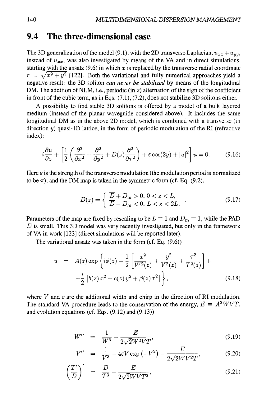
9.4 The three-dimensional case

The 3D generalization of the model (9.1), with the 2D transverse Laplacian,

Uxx

+Uyy,

instead of w^x, was also investigated by means of the VA and in direct simulations,

starting with the ansatz (9.6) in which x is replaced by the transverse radial coordinate

r =

A/X^

+ 2/2

[122].

Both the variational and fully numerical approaches yield a

negative result: the 3D soliton can never be stabilized by means of the longitudinal

DM. The addition of

NLM,

i.e., periodic (in z) alternation of the sign of the coefficient

in front of the cubic term, as in Eqs. (7.1), (7.2), does not stabilize 3D solitons either.

A possibility to find stable 3D solitons is offered by a model of a bulk layered

medium (instead of the planar waveguide considered above). It includes the same

longitudinal DM as in the above 2D model, which is combined with a transverse (in

direction y) quasi-ID lattice, in the form of periodic modulation of the RI (refractive

index):

w = 0. (9.16)

Here e is the strength of

the

transverse modulation (the modulation period is normalized

to be

TT),

and the DM map is taken in the symmetric form (cf. Eq. (9.2),

^^'^^[D-D^<Q,L<Z<2L,

• ^^-^^^

Parameters of the map are fixed by rescaling to be i = 1 and £)m = 1, while the PAD

D is small. This 3D model was very recently investigated, but only in the framework

in work [123] (direct simulations will be reported later).

The variational ansatz was taken in the form (cf. Eq. (9.6))

[1/^2 92 „, , 92 \ , , , „1

[2(^

^+''^'^^J''""^''^

+ '"'1

u = A{z) exp

•^ i(f>{z) —

2/2

+ T7TrT +

W2(z) v'^{z) T'2{z)_

+ '-[b{z)x^ + ciz)y^ + l3{z)T^]Y (9.18)

where V and c are the additional width and chirp in the direction of RI modulation.

The standard VA procedure leads to the conservation of the energy, E = A'^WVT,

and evolution equations (cf. Eqs. (9.12) and (9.13))

1 rp

W" = — — (9 19)

2V2W^VT'

^ • '

V" = :^ - AeVexp (-V^) ^^ ^ , (9.20)

T'\ D E

Dj T3

2V2WVT^'

(9.21)

9.4. THE THREE-DIMENSIONAL CASE 141

supplemented by the same matching (boundary) condition (9.14) as in the 2D model,

and also by the relations (cf. Eq. (9.11))

W V T'

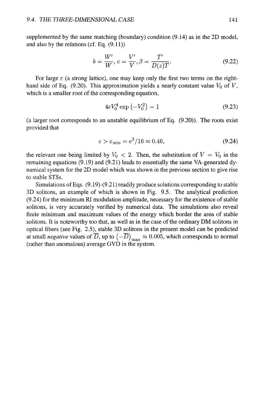
For large e (a strong lattice), one may keep only the first two terms on the right-

hand side of Eq. (9.20). This approximation yields a nearly constant value

of V,

which is a smaller root of the corresponding equation,

4sVo^exp{-Vo^)=l (9.23)

(a larger root corresponds to an unstable equilibrium of Eq. (9.20)). The roots exist

provided that

£ > £min = eVl6 « 0.46, (9.24)

the relevant one being limited by

< 2. Then, the substitution of ^ =

in the

remaining equations (9.19) and (9.21) leads to essentially the same VA-generated dy-

namical system for the 2D model which was shown in the previous section to give rise

to stable STSs.

Simulations of

Eqs.

(9.19)-(9.21) readily produce solutions corresponding to stable

3D solitons, an example of which is shown in Fig. 9.5. The analytical prediction

(9.24) for the minimum RI modulation amplitude, necessary for the existence of stable

solitons, is very accurately verified by numerical data. The simulations also reveal

finite minimum and maximum values of the energy which border the area of stable

solitons. It is noteworthy too that, as well as in the case of the ordinary DM solitons in

optical fibers (see Fig. 2.5), stable 3D solitons in the present model can be predicted

at small negative values of D, up to (—D) ~ 0.005, which corresponds to normal

(rather than anomalous) average GVD in the system.