Malomed B.A. Soliton Management in Periodic Systems

Подождите немного. Документ загружается.

152

FESHBACH RESONANCE IN OPTICAL LATTICES

100

' 5

- iu 1 i/q,

' max' 1 -1

mum

m mm

-A-

150

200

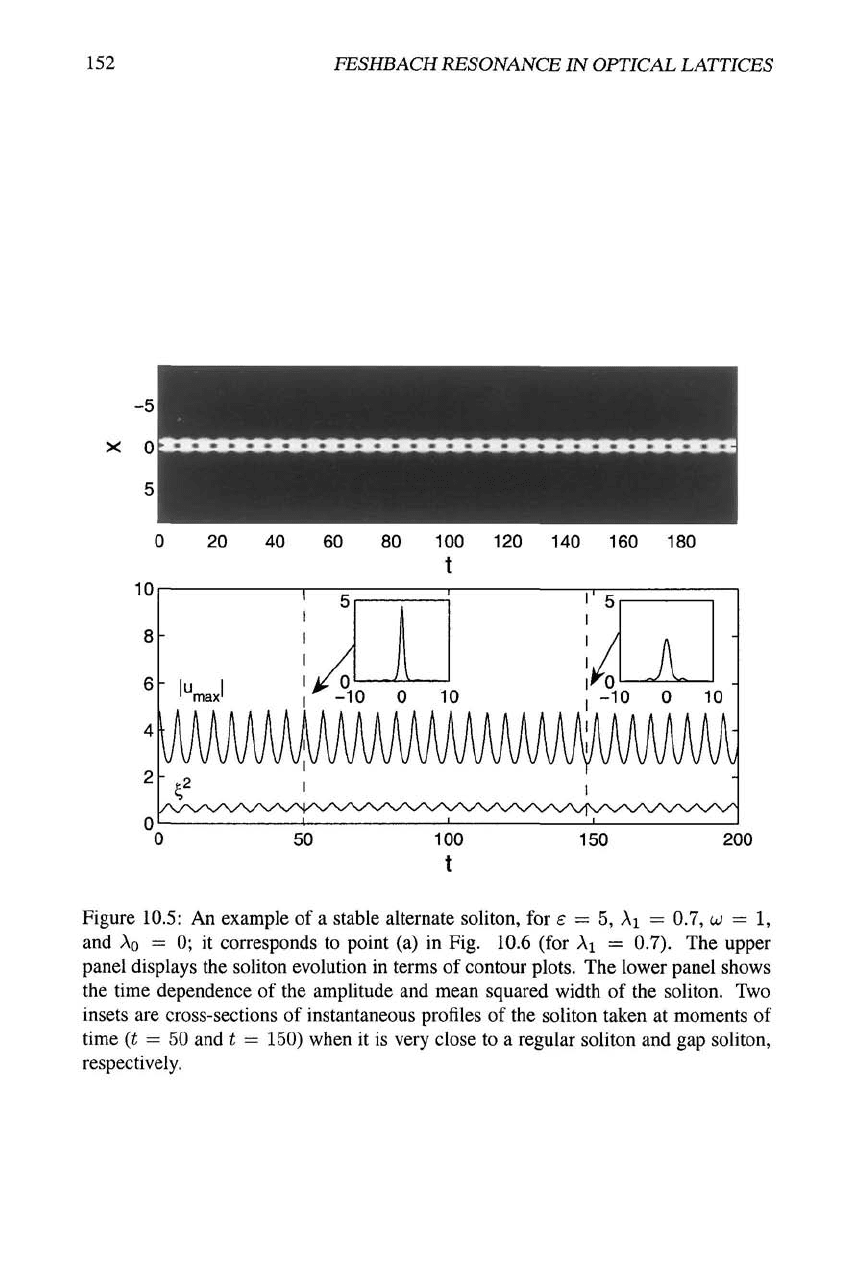
Figure 10.5: An example of a stable alternate soliton, for £ = 5, Ai = 0.7, w = 1,

and Ao = 0; it corresponds to point (a) in Fig. 10.6 (for Ai = 0.7). The upper

panel displays the soliton evolution in terms of contour plots. The lower panel shows

the time dependence of the amplitude and mean squared width of the soliton. Two

insets are cross-sections of instantaneous profiles of the soliton taken at moments of

time {t = 50 and t = 150) when it is very close to a regular soliton and gap soliton,

respectively.

10.3.

ALTERNATE REGULAR-GAP SOLITONS

153

4.5

3.5

3 2.5

1.5

0.51-

UNSTABLE

(b)x

A^=0.3 /

y^{^)<\J

/c) O

A^=o.5 y"^'

\ / \.

^=0-''

Energy Loss

by Radiation

<2%

3 4 5

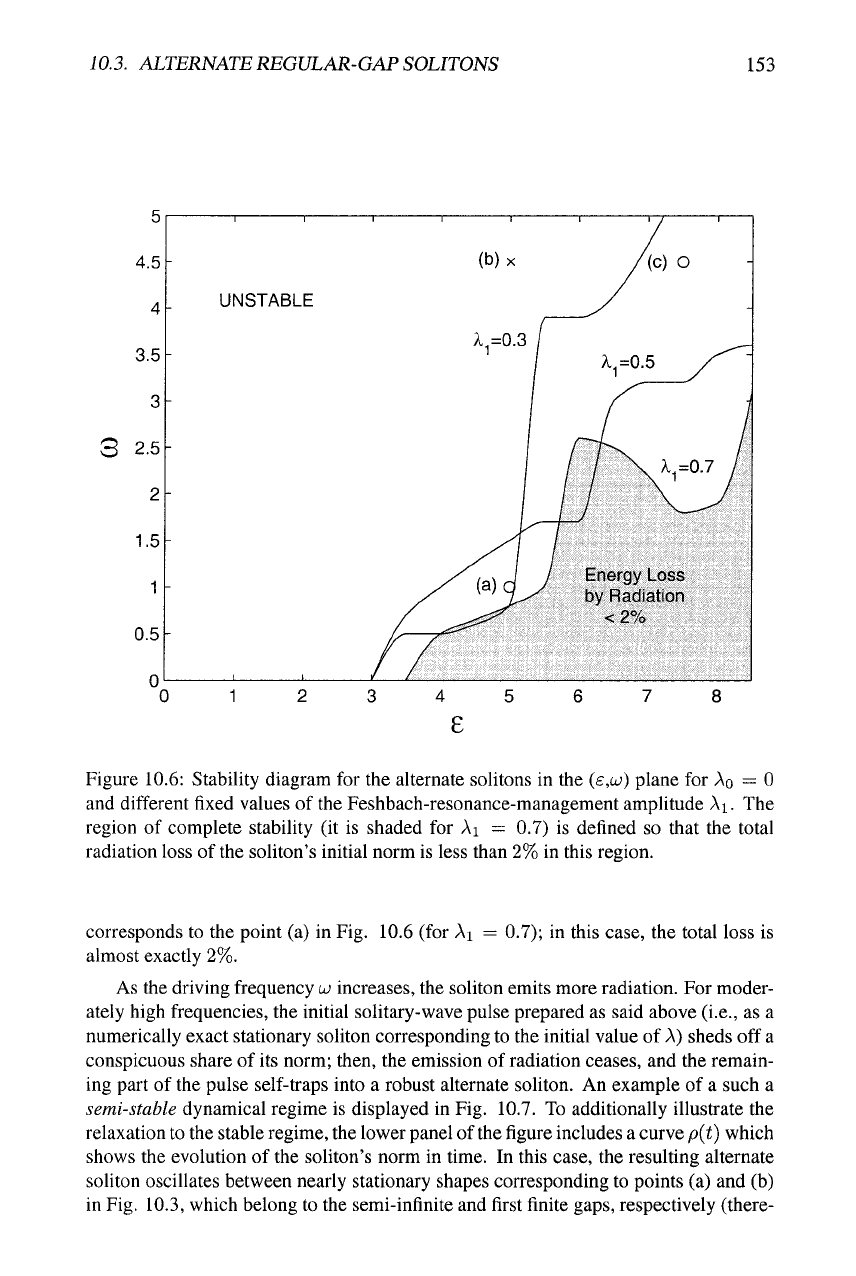
Figure 10.6: Stability diagram for the alternate solitons in the (£,c<;) plane for

= 0

and different fixed values of the Feshbach-resonance-management amplitude Ai. The

region of complete stability (it is shaded for Ai = 0.7) is defined so that the total

radiation loss of the soliton's initial norm is less than 2% in this region.

corresponds to the point (a) in Fig. 10.6 (for Ai = 0.7); in this case, the total loss is

almost exactly 2%.

As the driving frequency

increases, the soliton emits more radiation. For moder-

ately high frequencies, the initial solitary-wave pulse prepared as said above (i.e., as a

numerically exact stationary soliton corresponding to the initial value of

sheds off

conspicuous share of its norm; then, the emission of radiation ceases, and the remain-

ing part of the pulse self-traps into a robust alternate soliton. An example of a such a

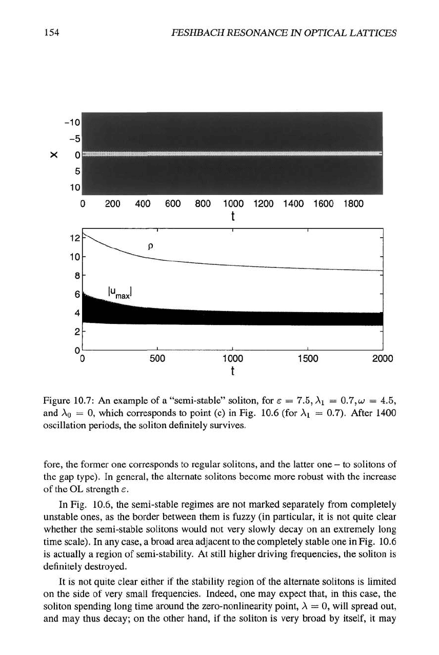
semi-stable dynamical regime is displayed in Fig. 10.7. To additionally illustrate the

relaxation to the stable regime, the lower panel of

the

figure includes a curve /j(t) which

shows the evolution of the soliton's norm in time. In this case, the resulting alternate

soliton oscillates between nearly stationary shapes corresponding to points (a) and (b)

in Fig. 10.3, which belong to the semi-infinite and first finite gaps, respectively (there-

154 FESHBACH RESONANCE IN OPTICAL LATTICES

200

400 600 800 1000 1200 1400 1600 1800

2000

Figure 10.7: An example of a "semi-stable" soliton, for s = 7.5, Ai = 0.7,

= 4.5,

and Ao = 0, which corresponds to point (c) in Fig. 10.6 (for Ai = 0.7). After 1400

oscillation periods, the soliton definitely survives.

fore,

the former one corresponds to regular solitons, and the latter one - to solitons of

the gap type). In general, the alternate solitons become more robust with the increase

of the OL strength e.

In Fig. 10.6, the semi-stable regimes are not marked separately from completely

unstable ones, as the border between them is fuzzy (in particular, it is not quite clear

whether the semi-stable solitons would not very slowly decay on an extremely long

time scale). In any case, a broad area adjacent to the completely stable one in Fig. 10.6

is actually a region of semi-stability. At still higher driving frequencies, the soliton is

definitely destroyed.

It is not quite clear either if the stability region of the alternate solitons is limited

on the side of very small frequencies. Indeed, one may expect that, in this case, the

soliton spending long time around the zero-nonlinearity point,

= 0, will spread out,

and may thus decay; on the other hand, if the soliton is very broad by

itself,

it may

10.3.

ALTERNATE REGULAR-GAP SOLITONS 155

survive this temporary spreading out. The lowest frequency checked in the simulations

was a; = 0.1, the solitons being unequivocally stable at this point.

It is also relevant to address the issue of the existence of the threshold necessary

for the formation of the soliton, which, as mentioned above, exists for both A > 0

and A < 0 in the static 2D models. In the nonstationary (FRM-driven) model with

the fixed norm (see Eq. (10.17)), rescaling (necessary to keep the norm fixed) shows

that the threshold manifests itself in the fact that persistent alternate solitons cannot be

found if the FRM-drive's amplitude is too small, Aj < (Ai)j.jjj,. In the strong lattice

with £ = 7.5 (the situation in the stationary model at this value of e is illustrated by

Figs.

10.3 and 10.4), the threshold exists but is so small that its accurate value cannot

be identified. This is possible for smaller e. In particular, for e = 4 it was found to be

(^i)thr ~ 0-^^' which should be compared to the the thresholds for the same £ = 4

and the same fixed norm (10.17) for the ordinary and gap solitons in the corresponding

static 2D models: x[lf^ w 0.04, and A^^^"^ » -0.04, respectively. Quite naturally,

the dynamical threshold is much higher than its static counterparts.

The FRM-driven soliton dynamics with a negative nonzero dc part of the nonlin-

earity coefficient,

< 0, which corresponds to repulsion, was also considered. The

interaction being repulsive on average, one may expect the existence of gap solitons in

the high-frequency limit. The situation may be illustrated by an example for

= —0.9

and Ai = 1.6. The simulations started with the initial profile corresponding to point

(a) in Fig. 10.3, as the initial value of the nonlinearity coefficient, A(0) = 0.7, pertains

to this point. The minimum instantaneous value of the oscillating nonlinear coefficient

is Amin = —2.5 in this case, the stationary solution with

= —2.5 pertaining to point

(d) in Fig. 10.3, which belongs to the second finite band. In this regime, the oscillating

nonlinear coefficient X{t), in addition to cycling across the point

= 0 and a very nar-

row Bloch band separating the semi-infinite and first finite gaps, periodically passes the

wider Bloch band between the first and the second finite gaps, where stationary soli-

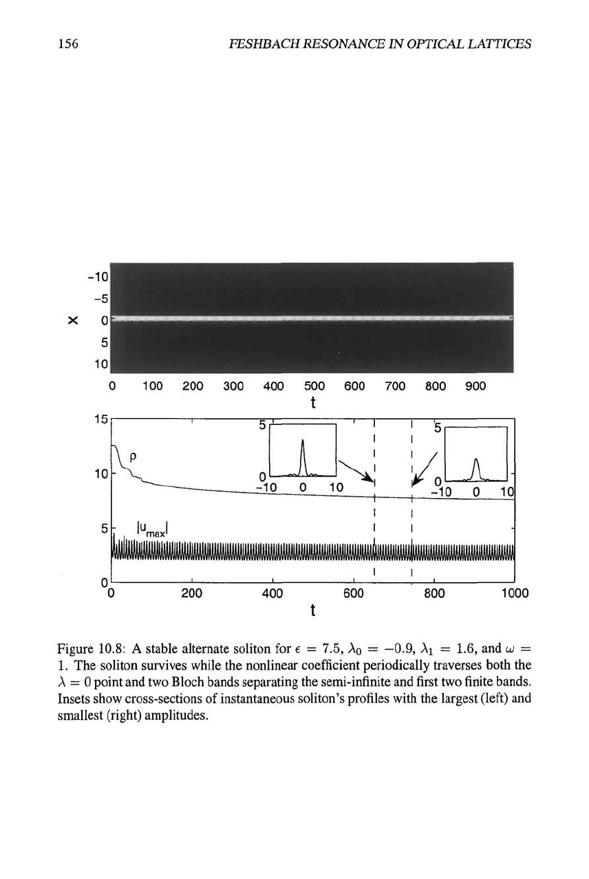
tons cannot exist. Nevertheless, a stable alternate soliton, found in this case, survives

all the traverses of the "dangerous zones", as shown in Fig. 10.8. A small amount of

radiation is emitted at the initial stage of the evolution (the curve p{t) again shows the

evolution of the soliton's norm), and then a robust alternate soliton establishes

itself,

cf. Fig. 10.7. It is noteworthy that, as seen in the insets, this soliton develops sidelobes

that actually do not oscillate together with its core, and do not disappear either as A

takes positive values. The latter feature distinguishes this stable regime from the one

shown in Fig. 10.5, where the sidelobes periodically disappear.

Finally, the application of the FRM mechanism to weakly localized ("loosely-

bound") solitons, such as the one in panel (f) of

Fig.

10.4, cannot produce any stable

regime periodically passing through a shape of this type, for any combination of

andAi inEq. (10.12).

10.3.3 Dynamics of one-dimensional solitons under the Feshbach-

resonance management

The ID case also deserves consideration, as the experiment may be easier in this case,

and it is interesting to compare the results with those reported above for the 2D model.

156

FESHBACH RESONANCE IN OPTICAL LATTICES

100 200 300 400 500 600 700 800 900

200 400 600

' t;

\ p

- V^,^^ Q

' \ It

' ' 5

1 1

•

^~--~ 3lO_0 10 1 ^_"io 0 10

T 1

1 1

- |u 1 II

1 . ' max'

1 1

1 r 1

800

1000

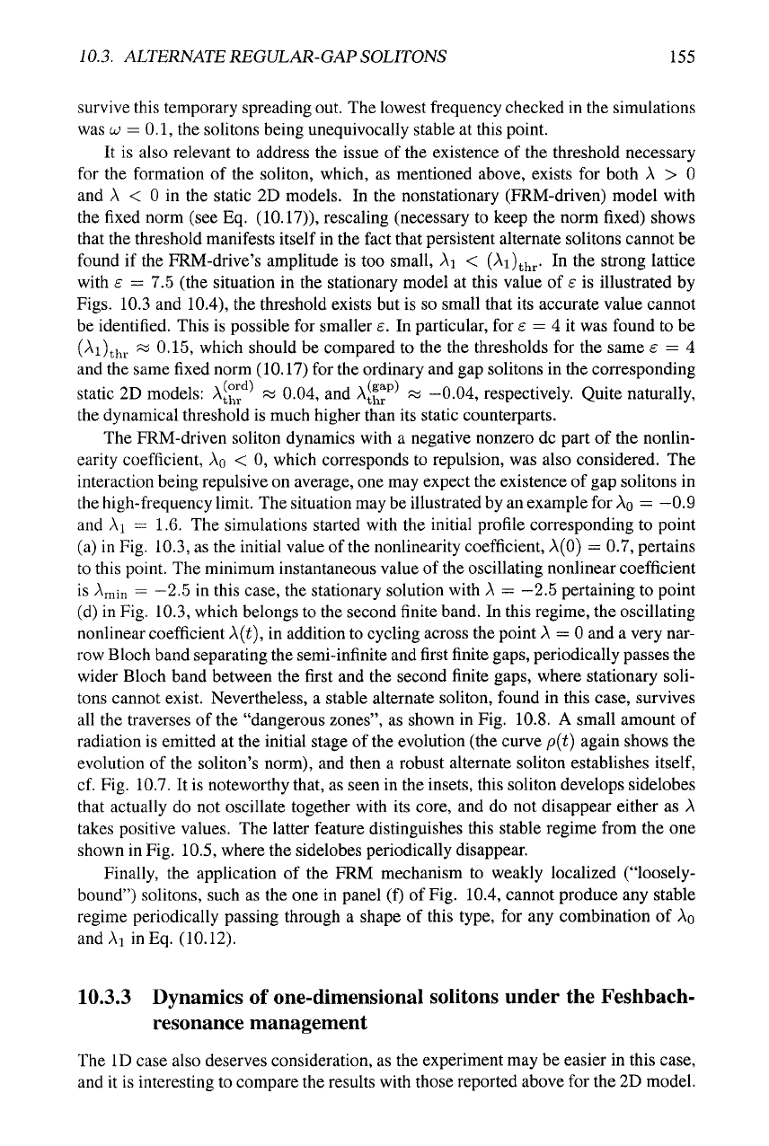
Figure 10.8: A stable alternate soliton for e = 7.5, Ao = —0.9, Ai = 1.6, and

The soliton survives while the nonlinear coefficient periodically traverses both the

= 0 point and two Bloch bands separating the semi-infinite and first two finite bands.

Insets show cross-sections of instantaneous soliton's profiles with the largest (left) and

smallest (right) amplitudes.

10.3.

ALTERNATE REGULAR-GAP SOLITONS 157

IliiiLilllii'

" 'Vc.

(a) (b)

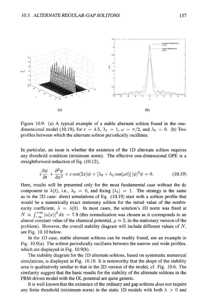
Figure 10.9: (a) A typical example of a stable alternate soliton found in the one-

dimensional model (10.19), for e = 4.5, Ai = 1, w = 7r/2, and Ao = 0. (b) Two

profiles between which the alternate soliton periodically oscillates.

In particular, an issue is whether the existence of the ID alternate soliton requires

any threshold condition (minimum norm). The effective one-dimensional GPE is a

straightforward reduction of

Eq.

(10.12),

i-^ + -Q^ + £cos(2x)V' + [Ao + Ai

cos{ujt)]

jVI^^ = 0. (10.19)

Here, results will be presented only for the most fundamental case without the dc

component in A(i), i.e.,

= 0, and fixing |Ai| = 1. The strategy is the same

as in the 2D case: direct simulations of Eq. (10.19) start with a soliton profile that

would be a numerically exact stationary soliton for the initial value of the nonlin-

earity coefficient, A = A(0). In most cases, the solution's ID norm was fixed at

N = f_°°

\u{x)\

dx — 7.9 (this normalization was chosen as it corresponds to an

almost constant value of the chemical potential,

« 2, in the stationary version of the

problem). However, the overall stability diagram will include different values of A^,

see Fig. 10.10 below.

In the ID case, stable alternate solitons can be readily found, see an example in

Fig. 10.9(a). The soliton periodically oscillates between the narrow and wide profiles,

which are displayed in Fig. 10.9(b).

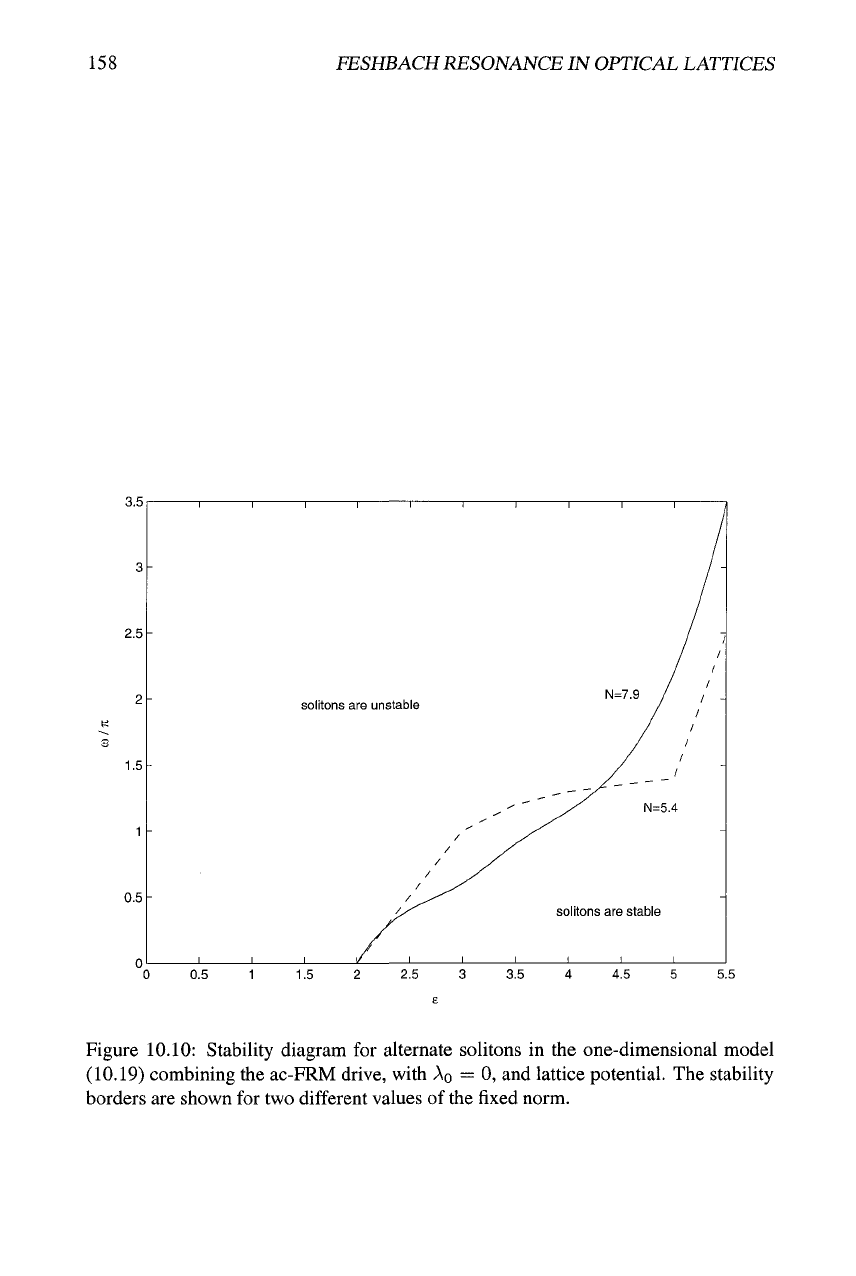
The stability diagram for the ID alternate solitons, based on systematic numerical

simulations, is displayed in Fig. 10.10. It is noteworthy that the shape of the stability

area is qualitatively similar to that in the 2D version of the model, cf. Fig. 10.6. The

similarity suggest that the basic results for the stability of the alternate solitons in the

FRM-driven model with the OL potential are quite generic.

It is well known that the existence of the ordinary and gap solitons does not require

any finite threshold (minimum norm) in the static ID models with both A > 0 and

158

FESHBACH RESONANCE IN OPTICAL LATTICES

3.5

2.5

1.5

0.5

solitons are unstable

0.5 1 1.5

Figure 10.10: Stability diagram for alternate solitons in the one-dimensional model

(10.19) combining the ac-FRM drive, with

= 0, and lattice potential. The stability

borders are shown for two different values of the fixed norm.

10.3.

ALTERNATE REGULAR-GAP SOLITONS 159

A < 0. A principal difference of

the

dynamic (FRM-driven) ID model is that persistent

alternate solitons can be found only above a finite

threshold,

N > A^thr- For instance,

the numerical results yield A^thr ~ 2.1 for e = 7.5 and a; = 7r/2. Thus, in this sense

the ID dynamic model is closer to the 2D one than to its static ID counterparts.

Besides the fundamental (single-peaked) ID solitons considered above, stable higher-

order (multi-peaked) alternate solitons can also be found in the FRM-driven ID model.

As concerns static higher-order solitons on lattices, a known example is the so-called

twisted localized mode, i.e., an odd (antisymmetric) soliton in the discrete NLS equa-

tion [45]. A similar object is a bound state of two lattice solitons, which, too, is stable

only in the anti-symmetric configuration, in the ID [84] and 2D [89] cases alike.

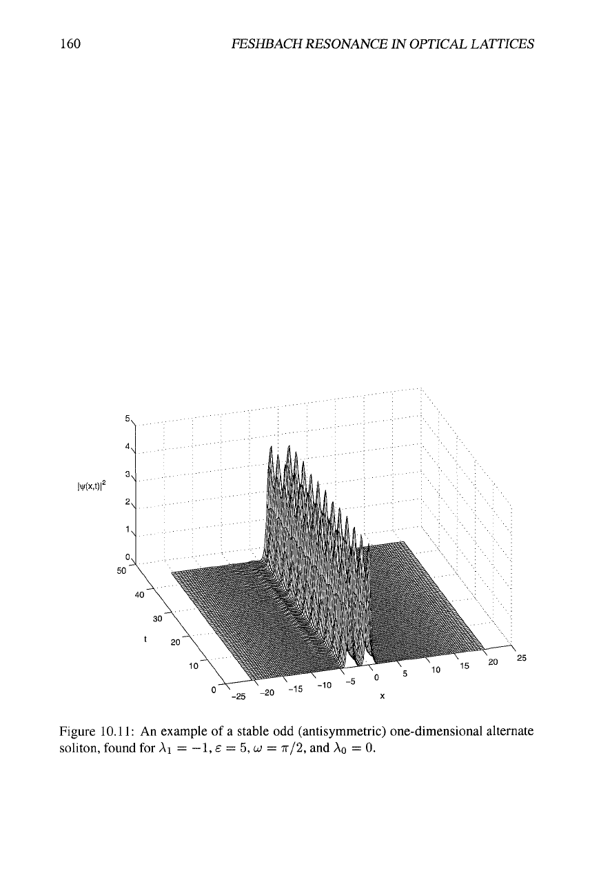
Following the pattern of the static lattice models, an antisymmetric initial state was

prepared as a superposition of two separated stationary solitons with opposite signs

(i.e.,

the phase difference

TT),

corresponding to the initial value of

. Direct simulations

demonstrate that stable alternate antisymmetric solitons can be easily found this way,

see a typical example in

Fig.

10.11.

Stable bound states of several fundamental solitons

with the phase shift

between them were found too in the present model.

A 2D counterpart of the odd soliton would be a vortical soliton. Such stable vortices

were found indeed in the static models with self-attraction [24, 174] and self-repulsion

[26,

152, 136]. However, simulations have not produced stable solitons with intrinsic

vorticity in the 2D FRM-driven model based on Eq. (10.12) with

—

160 FESHBACH RESONANCE IN OPTICAL LATTICES

i¥(x,t)r

••

-f-,-...iOi.r,,. ,

JT'*:^

-v^v^.

•/'.

"^M

•i:^,j'.

X-./-. M,h

• In 'v

"•

--•.'A'Vv

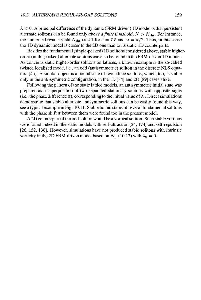
Figure

10.11:

An example of a stable odd (antisymmetric) one-dimensional alternate

soliton, found for Ai

—

5, w

TT/2,

and

= 0.

Bibliography

[1] F. Kh. Abdullaev and

B. Baizakov, Disintegration of a soliton in a dispersion-

managed optical communication line with

random

parameters, Opt. Lett. 25, 93

(2000).

[2] F. Kh. Abdullaev, B. B. Baizakov, and M. Salerno, Stable two-dimensional

dispersion-managed soliton, Phys. Rev. E 68,066605 (2003).

[3] F. Kh. Abdullaev and J. G. Caputo, Validation of

the

variational approach for

chirped pulses in fibers with periodic dispersion, Phys. Rev. E 58, 6637 (1998).

[4] F. Kh. Abdullaev, J. G. Caputo, and N. Flytzanis, Envelope soliton propagation

in media with temporally modulated dispersion, Phys. Rev. E 50, 1552 (1994).

[5] F Kh. Abdullaev, J. G. Caputo, R. A. Kraenkel, and

A. Malomed, Controlling

collapse

Bose-Einstein condensation by

temporal

modulation of the scattering

length, Phys. Rev. A 67, 013605 (2003).

[6] F Kh. Abdullaev and R. Galimzyanov, The dynamics of bright matter wave

solitons in a quasi-one-dimensional Bose-Einstein condensate with a rapidly

varying trap, J. Phys. B 36, 1099 (2003).

[7] F. Kh. Abdullaev and J. Garnier, Collective oscillations of one-dimensional

Bose-Einstein gas in a time-varying

trap

potential and atomic scattering length,

Phys.

Rev. A 70,053604 (2004).

[8] F. Kh. Abdullaev and P. K. KhabibuUaev. Dynamics of Solitons in Inhomoge-

neous Condensed Media (Fan Publishers: Tashkent, 1986) (in Russian).

[9] M. J. Ablowitz and G. Biondini, Multiscale pulse dynamics in communica-

tion systems with strong dispersion management. Opt. Lett. Opt. Lett. 23, 1668

(1998).

[10] M. J. Ablowitz, G. Biondini, S. Chakravarty, and R. L. Home, On timing

jit-

ter in wavelength-division multiplexed soliton systems. Opt. Commun. 150, 305

(1998).

[11] M. Ablowitz and H. Segur. Solitons and the Inverse Scattering Transform

(SIAM: Philadelphia, 1981).