Malomed B.A. Soliton Management in Periodic Systems
Подождите немного. Документ загружается.

142 MULTIDIMENSIONAL DISPERSION MANAGEMENT
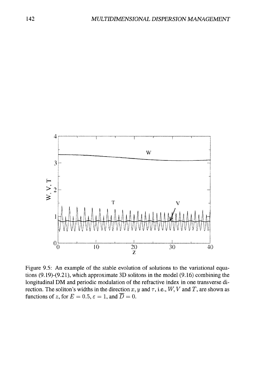
Figure 9.5: An example of the stable evolution of solutions to the variational equa-
tions (9.19)-(9.21), which approximate 3D solitons in the model (9.16) combining the
longitudinal DM and periodic modulation of the refractive index in one transverse di-
rection. The soliton's widths in the direction x, y and r, i.e., W, V and T, are shown as
functions of z, for E = 0.5, £ = 1, and D = 0.
Chapter 10
Feshbach-resonance
management in optical lattices
10.1 Introduction to the topic
Stabilization of 3D solitons in nonlinear optics and BECs (Bose-Einstein condensates)
is a cardinal problem in the current studies in these fields. Various theoretical ap-
proaches to this topic constitute one of central themes of the present book. As ex-
plained in previous chapters, the ac-FRM technique, in the form of periodic reversal
of the sign in front of the nonlinear terms in the corresponding GPE (Gross-Pitaevskii
equation), is sufficient to stabilize only 2D solitons in
BEC.
On the other hand, a quasi-
ID optical lattice (OL), which is much easier to create in the experiment than its multi-
dimensional (2D or 3D) counterparts, is also capable to support stable solitons only in
the 2D setting, but not in three dimensions [26]. These findings suggest a natural ques-
tion, whether a combination of FRM and quasi-ID lattice may be sufficient to stabilize
3D solitons. In a recent work [166] a positive answer was given to this question, using
an analytical approach (VA) and direct simulations.
The interplay of an OL and low-frequency FRM suggests another interesting pos-
sibility. Indeed, it is well known that the GPE equipped with the OL gives rise to
regular solitons or GSs (gap solitons) if the nonlinearity is, respectively, self-attractive
or self-repulsive. Then, in the case of periodic slow switching between the two signs
of the nonlinearity provided by the FRM, a question arises, whether periodic adiabatic
transitions between solitons of the two types can be predicted. The corresponding sta-
ble alternate solitons are possible indeed, as was demonstrated in both the 2D and ID
settings [77]. An account of these results is also included in the present chapter.
144 FESHBACH RESONANCE IN OPTICAL LATTICES
10.2 Stabilization of three-dimensional solitons by the
Feshbach-resonance management in a quasi-one-
dimensional lattice
10.2.1 The model and variational approximation
The model introduced in work [166] is based on the GPE in three dimensions, that
includes the ID lattice potential and the same ac-FRM modulation of the nonlinearity
coefficient as in other models considered in this book. Thus, the normalized equation
for the single-particle wave function
tp
is
--V'
+ £ (1 - cos(2z)) +
{go
+ gi sin(Ot)) jV'l^
V',
(10.1)
where the Laplacian (kinetic-energy operator) V'^ acts on all the three coordinates x, y,
and z. Further, e is the strength of the OL potential, whose period is scaled to be
TT,
go
and gi account for the dc and ac parts of the FRM-controUed nonlinearity coefficient,
and
D.
is the ac-FRM frequency. Solitons can be constructed only in the case of
50
< 0,
which implies that the constant part of the interaction is self-attractive.
Equation (10.1) can be derived from the Lagrangian,
L =
+00
dz
-2£(1
gdg
008(2^)) IV-I
(5o+3isin(f2i))IV'l']
d'lP
dg
2
dz
(10.2)
where the asterisk stands for the complex conjugation, and g = ^Jx^
-\-
y^ is the radial
variable in the plane transverse to the lattice. To apply the VA to this model, a complex
Gaussian ansatz may be adopted (cf., for instance, ansatz (9.6), with the real amplitude
^(i),
phase 0(^), radial and axial widths W{t) and V{i), and the corresponding chirps
6(Oand/3(t):
ip{r,t) = Aexp
2W^
+ ib
(J-
+
if3
(10.3)
An effective Lagrangian is obtained by inserting the ansatz (10.3) into Eq. (10.2). The
Euler-Lagrange equations derived from the effective Lagrangian yield, first, the con-
servation of the solution's norm (dE/dt = 0), which is proportional to the number of
atoms in the condensate,
E =
—
Id r
^ J-00 Jo
gdg\^\^ =
A^W^V,
(10.4)
and dynamical equations for the widths W and V (cf. Eqs. (9.13), (9.12), derived in a
similar situation in the previous chapter):
fW_ _ _1_ E
dt^
d^V
df^
Vsww
[90
+ 5i sin(r2t)],
(10.5)
1
__ = __4£Fexp(-y2)
E
V8iy2y2
[go
+ gism{nt)]. (10.6)
10.2.
STABILIZATION OF THREE-DIMENSIONAL SOLITONS 145
Numerical results will be given below for the normalization E
—
TT"^/^ (this condition
may always be imposed by rescaling g^ and gi).
A necessary condition for the existence of a 3D soliton in the present model can be
derived from these equations in an approximate form. To this end, it is assumed that gi
is small, while Q is large in Eq. (10.1). It is also conjectured that the average value W
of the soliton's radial size, W, is large (see below). Further, in the lowest approxima-
tion, the soliton's size in the axial direction may be assumed constant, V{t) w
VQ,
as
determined by the relation
AsVo^exp{-V^)=l, (10.7)
that follows from Eq. (10.6) where the last small term (~ W^"^) is dropped. Equa-
tion (10.7) has real solutions if the OL strength exceeds a minimum (threshold) value,
e > ethr = eVl6 « 0.46 (10.8)
(note the same value appeared in a similar context in the model considered in the pre-
vious chapter, see Eq. (9.24)). For s > Sthr, Eq. (10.7) has two real solutions, which
implies the existence of two different solitons. It seems very plausible (cf. the situation
for static models considered
Refs.
[24,25,26]) that the narrower soliton, corresponding
to smaller
VQ,
is stable, and the other one is unstable.
Next, replacing V(t) by
VQ
in Eq. (10.6), one may look for a solution as W{t) w
W + Wi sin
(fit).
For large fl, the variable part of the equation yields
Wi = ^ . (10.9)
Then, the consideration of the constant part of Eq. (10.5), with regard to the first cor-
rection generated by averaging of the product of Wi sin (ilt) g{t), yields the following
result:
W' = -±- (^)\ , ' ^ , . (10.10)
4v^yo \ ^ J {E\go\-V8Vo) '
An essential corollary of Eq. (10.10) is a necessary condition for the existence of the
3D soliton:
\9\>{\9o\U^
= ^ (10.11)
(recall ^o is negative). In fact, this minimum value, for given E, corresponds (within
the framework of the VA) to the critical norm necessary for the existence of the 2D
soliton (i.e., the norm of the TS). Direct simulations presented in the next subsection
show that this condition holds indeed, albeit approximately.
4
Finally, the above conjecture, that W is large, is (formally) valid only when l^ol
slightly exceeds the minimum value defined in Eq. (10.11) - then, the expression
(10.10) will be large, as the denominator is small.
146 FESHBACH RESONANCE
IN
OPTICAL LATTICES
'.
M
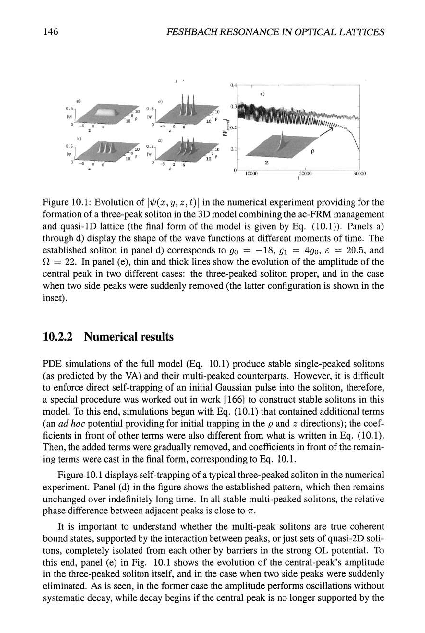
Figure 10.1: Evolution
of
\i){x,
y, z, t)\ in the
numerical experiment providing
for the
formation
of
a
three-peak soliton
in the
3D model combining
the
ac-FRM management
and quasi-lD lattice
(the
final form
of the
model
is
given
by Eq.
(10.1)). Panels
a)
through
d)
display
the
shape
of
the wave functions
at
different moments
of
time.
The
established soliton
in
panel
d)
corresponds
to
go
=
—18,
gi = igo, e — 20.5, and
Vt
= 22. In
panel
(e),
thin
and
thick lines show
the
evolution
of the
amplitude
of the
central peak
in two
different cases:
the
three-peaked soliton proper,
and in the
case
when
two
side peaks were suddenly removed
(the
latter configuration
is
shown
in the
inset).
10.2.2 Numerical results
PDE simulations
of the
full model
(Eq. 10.1)
produce stable single-peaked solitons
(as predicted
by the
VA)
and
their multi-peaked counterparts. However,
it is
difficult
to enforce direct self-trapping
of an
initial Gaussian pulse into
the
soliton, therefore,
a special procedure
was
worked
out in
work
[166] to
construct stable solitons
in
this
model.
To
this
end,
simulations began with Eq. (10.1) that contained additional terms
(an
ad hoc
potential providing
for
initial trapping
in the
Q
and z
directions);
the coef-
ficients in front
of
other terms were also different from what
is
written
in Eq.
(10.1).
Then,
the
added terms were gradually removed,
and
coefficients
in
front
of
the remain-
ing terms were cast
in the
final form, corresponding to Eq.
10.1.
Figure 10.1 displays self-trapping
of
a
typical three-peaked soliton
in
the numerical
experiment. Panel
(d) in the
figure shows
the
established pattern, which then remains
unchanged over indefinitely long time.
In all
stable multi-peaked solitons,
the
relative
phase difference between adjacent peaks
is
close
to
TT.
It
is
important
to
understand whether
the
multi-peak solitons
are
true coherent
bound states, supported
by the
interaction between peaks, or just sets
of
quasi-2D soli-
tons,
completely isolated from each other
by
barriers
in the
strong
OL
potential.
To
this
end,
panel
(e) in Fig. 10.1
shows
the
evolution
of the
central-peak's amplitude
in
the
three-peaked soliton
itself, and in the
case when
two
side peaks were suddenly
eliminated.
As is
seen,
in the
former case
the
amplitude performs oscillations without
systematic decay, while decay begins
if
the central peak
is no
longer supported
by the
10.2.
STABILIZATION OF THREE-DIMENSIONAL SOLITONS
147
I '
+ +
+ + + + + ++•+ + +
+++++++++++
+++++++++++
•+++++++++++
•+++++++++++
•+++++++++++
+++++++++++
- - + + + + + + + + +
'• ••
''•••+
+ + + + +
VA:
I I
stabilily Numerics:
"^
stabilitv
^ cflllapse ^ spread our » collapse r^ spread oul
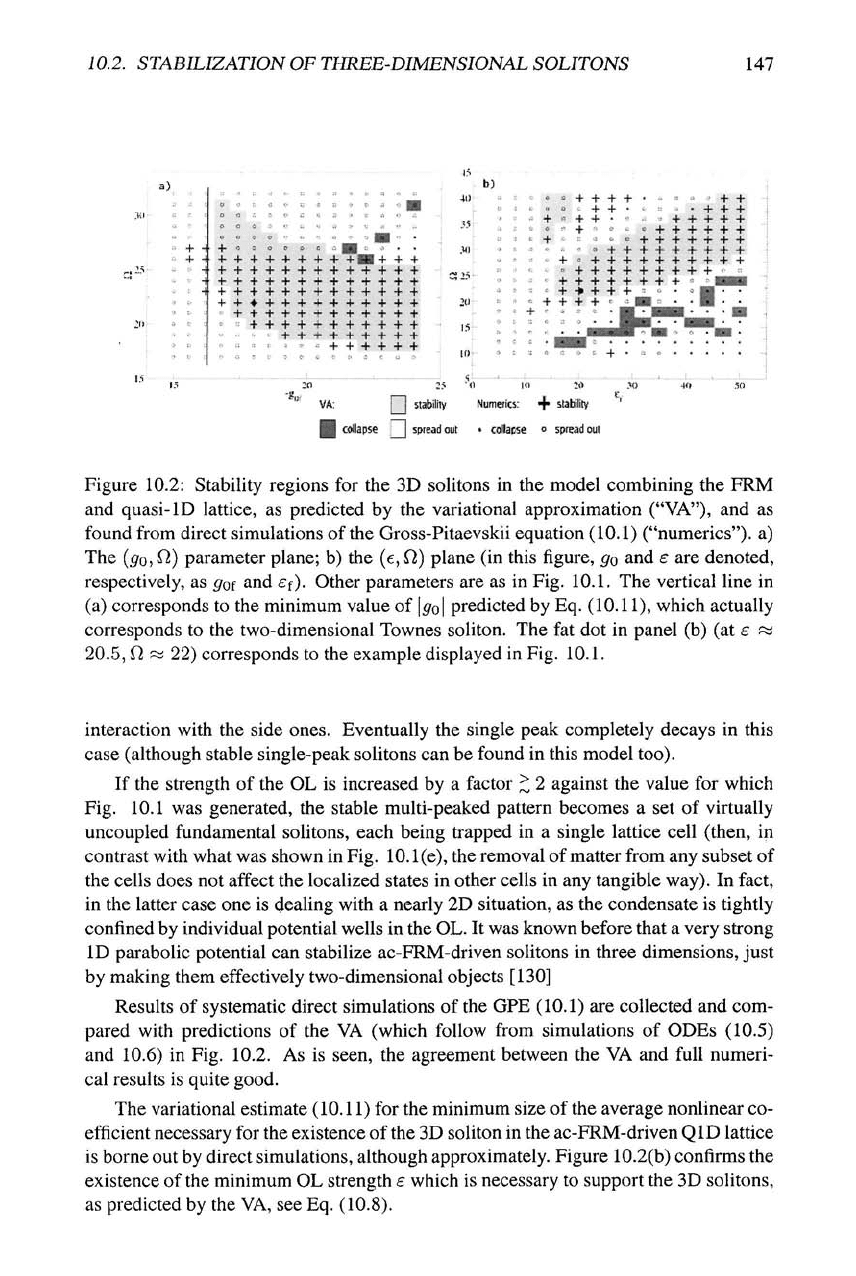
Figure 10.2: Stability regions for the 3D solitons in the model combining the FRM
and quasi-ID lattice, as predicted by the variational approximation ("VA"), and as
found from direct simulations of the Gross-Pitaevskii equation (10.1) ("numerics"), a)
The
{go,
f2) parameter plane; b) the (e,
Q,)
plane (in this figure, go and s are denoted,
respectively, as goi and ef). Other parameters are as in Fig. 10.1. The vertical line in
(a) corresponds to the minimum value of
\go\
predicted by Eq. (10.11), which actually
corresponds to the two-dimensional Townes soliton. The fat dot in panel (b) (at e w
20.5,
Q w 22) corresponds to the example displayed in Fig. 10.1.
interaction with the side ones. Eventually the single peak completely decays in this
case (although stable single-peak solitons can be found in this model too).
If the strength of the OL is increased by a factor ^ 2 against the value for which
Fig. 10.1 was generated, the stable multi-peaked pattern becomes a set of virtually
uncoupled fundamental solitons, each being trapped in a single lattice cell (then, in
contrast with what was shown in
Fig. 10.1 (e),
the removal of matter from any subset of
the cells does not affect the localized states in other cells in any tangible way). In fact,
in the latter case one is dealing with a nearly 2D situation, as the condensate is tightly
confined by individual potential wells in the OL. It was known before that a very strong
ID parabolic potential can stabilize ac-FRM-driven solitons in three dimensions, just
by making them effectively two-dimensional objects [130]
Results of systematic direct simulations of the GFE (10.1) are collected and com-
pared with predictions of the VA (which follow from simulations of ODEs (10.5)
and 10.6) in Fig. 10.2. As is seen, the agreement between the VA and full numeri-
cal results is quite good.
The variational estimate (10.11) for the minimum size of the average nonlinear co-
efficient necessary for the existence of the 3D soliton in the ac-FRM-driven QID lattice
is borne out by direct simulations, although approximately. Figure 10.2(b) confirms the
existence of the minimum OL strength e which is necessary to support the 3D soHtons,
as predicted by the VA, see Eq. (10.8).
148 FESHBACH RESONANCE IN OPTICAL LATTICES
10.3 Alternate regular-gap solitons in one- and
two-dimensional lattices under the ac
Feshbach-resonance drive
10.3.1 The model
The model dealt with in this section is set in the 2D space with a full 2D lattice. The
corresponding GPE is
i^ + ^ + ^ + £ [cos(2x) + cos(2y)] V +
[AQ
+ Ai cos(wt)] IV'lV = 0,
(10.12)
The only dynamical invariant of Eq. (10.12) (with the time-dependent nonlinearity
coefficient) is the norm, which is proportional
to
the number of
atoms
in the condensate,
N= I [ \i;{x,y,t)f dxdy. (10.13)
The objective of the consideration is to find alternate solitons, which perform periodic
adiabatic transitions between gap-soliton configurations and regular solitons that cor-
respond, respectively, to
AQ
+ Ai cos(wt) < 0 and
AQ
+ Ai cos(a;t) > 0, in the case
when the modulation frequency
OJ
is small enough. The results included in this section
were obtained in work [77].
In case of
Aj
= 0, stationary solutions to Eq. (10.12) are sought as
'4'{x,y,t) = u{x,y)exp{-int), (10.14)
with a real chemical potential /i and a real function u which satisfies the equation
d Vj d u
MW
+ ^ + ^ + £ [cos(2x)
-I-
cos(2y)] u +
XQU^
= 0. (10.15)
Search for soliton solutions should be preceded by consideration of
the
spectrum of the
linearized version of Eq. (10.15), as solitons may only exist at values of
/j.
belonging
to bandgaps in the spectrum. The linearization of
Eq.
(10.15) leads to a separable 2D
eigenvalue problem,
[L:c + Ly\u{x,y) =-^u{x,y), (10.16)
where a ID linear operator is Lx = d'^ jdx^
-\-
£cos(2a;). The corresponding eigen-
states can be built as Uki{x,y) = gk{x)gi{y), with the eigenvalues iiki =
/J-k
+
jJ-i,
where gk{x) and gi{y) is any pair of quasi-periodic Bloch functions solving the linear
ME (Mathieu equation), Lxgkix) =
—fJ.kgk{x),
fJ-k
and fii being the corresponding
eigenvalues. The band structure of the 2D linear equation (10.16) constructed this way
was already investigated in detail (see, e.g., papers [135] and [56]). It includes, as
the spectrum of the ME
itself,
a semi-infinite gap which extends to /i
—>
—
oo,
and a
10.3.
ALTERNATE REGULAR-GAP SOLITONS
149
c<
-5
-6
-7
-20
semi-infinite gap
\ \
"^ '
m
/
-15
-10 -5
10
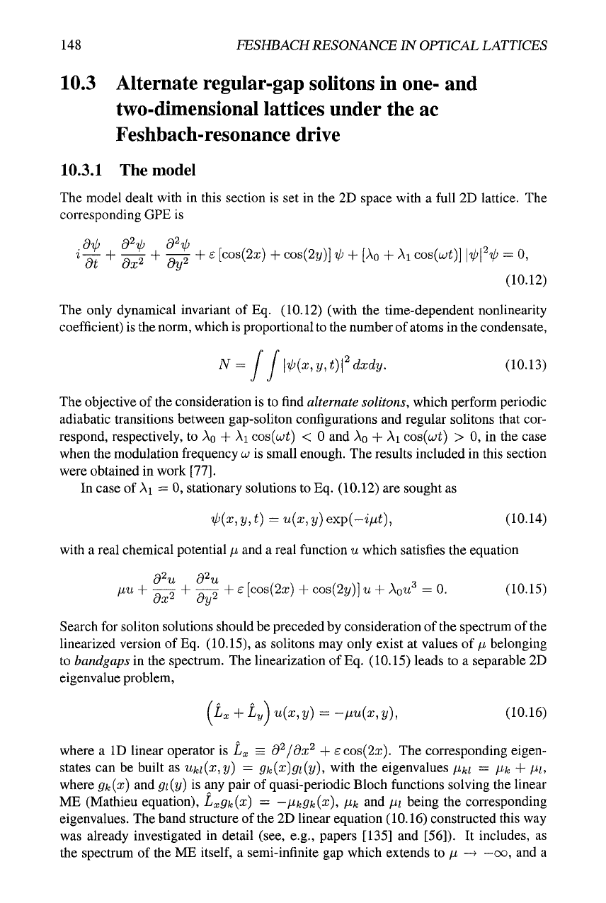
Figure 10.3: The system of vertical stripes gives a typical example (for e = 7.5) of
the bandgap structure found from the linearized version of Eq. (10.15), shaded and
unshaded zones being the Bloch bands and gaps, respectively (solitons may exist only
inside the gaps). The solid curve shows the dependence /^(AQ) for numerical soli-
ton solutions, as found (also for e = 7.5, and for a fixed norm, A'' = 47r) from the
full nonlinear stationary equation (10.15). The dashed curve is the same dependence
for approximate soliton solutions found by means of a variational method based on a
Gaussian ansatz (details of the latter are given in paper [77]). Points "a" through "f'
mark particular solitons whose shapes are given in Fig. 10.4.
150 FESHBACH RESONANCE IN OPTICAL LATTICES
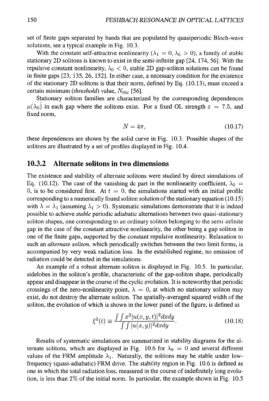
set of finite gaps separated by bands that are populated by quasiperiodic Bloch-wave
solutions, see a typical example in Fig. 10.3.
With the constant self-attractive nonlinearity (Aj = 0,
AQ
> 0), a family of stable
stationary 2D solitons is known to exist in the semi-infinite gap [24, 174, 56]. With the
repulsive constant nonlinearity,
AQ
< 0, stable 2D gap-soliton solutions can be found
in finite gaps [23, 135, 26, 152]. In either case, a necessary condition for the existence
of the stationary 2D solitons is that their norm, defined by Eq. (10.13), must exceed a
certain minimum (threshold) value, A^thr [56].
Stationary soliton families are characterized by the corresponding dependences
/Li(Ao) in each gap where the solitons exist. For a fixed OL strength e = 7.5, and
fixed norm,
A'' = 47r, (10.17)
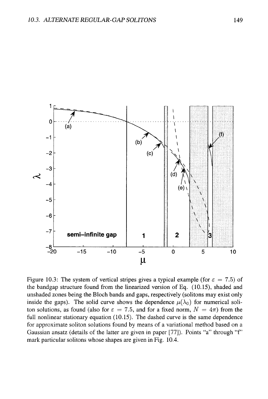
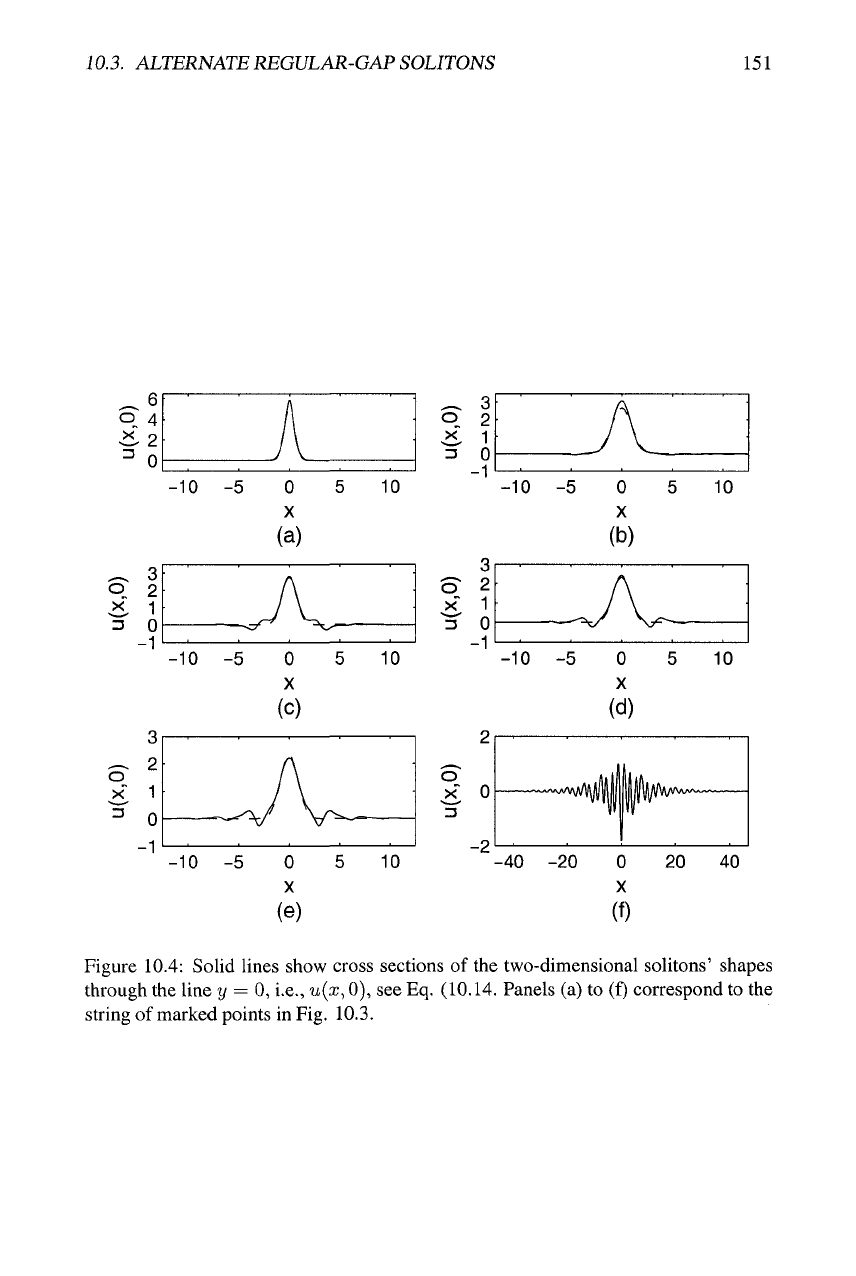
these dependences are shown by the solid curve in Fig. 10.3. Possible shapes of the
solitons are illustrated by a set of profiles displayed in Fig. 10.4.
10.3.2 Alternate solitons in two dimensions
The existence and stability of alternate solitons were studied by direct simulations of
Eq. (10.12). The case of the vanishing dc part in the nonlinearity coefficient,
AQ
=
0, is to be considered first. At i = 0, the simulations started with an initial profile
corresponding to a numerically found soliton solution of the stationary equation (10.15)
with
A
= Aj (assuming Ai > 0). Systematic simulations demonstiate that it is indeed
possible to achieve stable periodic adiabatic alternations between two quasi-stationary
soliton shapes, one corresponding to an ordinary soliton belonging to the semi-infinite
gap in the case of the constant attractive nonlinearity, the other being a gap soliton in
one of the finite gaps, supported by the constant repulsive nonlinearity. Relaxation to
such an alternate soliton, which periodically switches between the two limit forms, is
accompanied by very weak radiation loss. In the established regime, no emission of
radiation could be detected in the simulations.
An example of a robust alternate soliton is displayed in Fig. 10.5. In particular,
sidelobes in the soliton's profile, characteristic of the gap-soliton shape, periodically
appear and disappear in the course of the cyclic evolution. It is noteworthy that periodic
crossings of the zero-nonlinearity point, A = 0, at which no stationary soliton may
exist, do not destroy the alternate soliton. The spatially-averaged squared width of the
soliton, the evolution of which is shown in the lower panel of the figure, is defined as
eit)
= S
! A<^.y^t)?d^dy
_
^^^^^^
f J
\u{x,y)\'^dxdy
Results of systematic simulations are summarized in stability diagrams for the al-
ternate solitons, which are displayed in Fig. 10.6 for
AQ
= 0 and several different
values of the FRM amplitude Ai. Naturally, the solitons may be stable under low-
frequency (quasi-adiabatic) FRM drive. The stability region in Fig. 10.6 is defined as
one in which the total radiation loss, measured in the course of indefinitely long evolu-
tion, is less than 2% of the initial norm. In particular, the example shown in Fig. 10.5
10.3.
ALTERNATE REGULAR-GAP SOLITONS
151
6
o 4
^2
3 r,
0
-10
^ 3
9-
2
3 0
-1 '—•—
-10
o
^ 2
o
X 1
^ 0
-1
-10
-5
<f
-5
—^
-5
A
/\
0
X
(a)
A
JV
0
X
(c)
A
0
X
(e)
5
\^
5
y~^^^
7 ^^
5
10
10
10
O
^
^
o"
^
^
3
2
1
0
-10
3
2
1
0
-1
1——
-10
0
-2
-40
-5
-^
-5
^•vWV^/J^f
-20
A
y
V
0
X
(b)
A
J\
0
X
(d)
•
0
X
(f)
5
y^—
5
^/\/\/\ftA/>~
20
10
•
10
40
Figure 10.4: Solid lines show cross sections of the two-dimensional solitons' shapes
through the line y = 0, i.e., u{x, 0), see Eq. (10.14. Panels (a) to (f) correspond to the
string of marked points in Fig. 10.3.