Malomed B.A. Soliton Management in Periodic Systems

Подождите немного. Документ загружается.

PREFACE

of one-dimensional settings, and the respective results, are very different from those

which are relevant to multidimensional problems (nevertheless, chapter 10 includes

some results for a one-dimensional situation too, which are closely related to the basic

two-dimensional problem which is considered in that chapter).

Writing this book would not be possible without valuable collaborations and dis-

cussions with a large number of colleagues. It is my great pleasure to express the

gratitude to F. Kh. Abdullaev, J. Atai, B. B. Baizakov, Y. B. Band, A. Berntson, J. G.

Caputo, A. R. Champneys,

P. Chen, P L. Chu, D. J. Frantzeskakis, B. V. Gisin, D.

J. Kaup, P G. Kevrekidis,

S. Kivshar, R. A. Kraenkel,

Lakoba, U. Mahlab, D. Mi-

halache,

Perez-Garcfa, M. Salerno, M. Segev, N. Smyth, L. Torner, M. Trippenbach,

Wise, and J. Yang. Special thanks are due to younger collaborators (some of them

were my students or postdoc associates), including R. Driben, A. Gubeskys, M. Gutin,

A. Kaplan, M. Matuszewski, T. Mayteevarunyoom,

I. Merhasin, G. Theocharis, and

I. Towers.

The work on particular projects that have generated essential results included in

this book was supported, in various forms and parts, by grants No. 1999459 from the

Binational (US-Israel) Science Foundation, and No. 8006/03 from the Israel Science

Foundation. At a smaller scale, support was also provided by the European Office of

Research and Development of the US Air Force, and Research Authority of the Tel

Aviv University.

xii PREFACE

List of acronyms used in the text:

ID,

2D, 3D - one-dimensional, two-dimensional, three-dimensional

AWG - antiwaveguide

BEC - Bose-Einstein condensation/condensate

BG - Bragg grating

CW - continuous-wave (solution)

DM - dispersion management

DS - dark soliton

FF - fundamental-frequency (wave)

FP - fixed point

FR - Feshbach resonance

FRM - Feshbach-resonance management

FWHM - full width at half-maximum (of an optical pulse)

FWM - four-wave mixing

OPE - Gross-Pitaevskii equation

GS - gap soliton

GVD - group-velocity dispersion

GVM - group-velocity mismatch

HS - hot spot (a local perturbation switching a spatial soliton)

ISI - inter-symbol interference

1ST - inverse-scattering transform

KdV - Korteweg - de Vries (equation)

ME - Mathieu equation

NLM - nonlinearity management

NLS - nonlinear Schrodinger (equation or soliton)'

ODE - ordinary differential equation

OL - optical lattice

PAD - path-average dispersion

PCF - photonic-crystal fiber

PDE - partial differential equation

PR - parametric resonance

QPM - quasi-phase-matching

RI - refractive index

RZ - retum-to-zero (signal)

SH - second harmonic

SHG - second-harmonic generation

SPM - self-phase modulation

SSM - split-step model

STS - spatiotemporal soliton

TF - Thomas-Fermi (approximation)

TS - Townes soliton

VA - variational approximation

WDM - wavelength-division multiplexing

WG - waveguide (when referred to in the context of the waveguding-antiwaveguiding model)

XPM - cross-phase modulation

Chapter 1

Introduction

1.1 An overview of the concept of solitons

The concept of solitons (solitary waves) plays a profoundly important role in modern

physics and applied mathematics, extending beyond the bounds of these disciplines. It

was introduced in 1965 by Zabusky and Kruskal who numerically simulated collisions

between solitary waves (pulses) in the Korteweg - de Vries (KdV) equation, and dis-

covered that these pulses not only are stable in isolation, but also completely recover

their shapes after collisions

[175];

this observation was an incentive which had soon

led to the discovery of the inverse scattering transform (1ST) and the very concept of

integrable nonlinear partial differential equations (PDEs) [72]. The next principally

important step in this direction was made by Zakharov and Shabat, who had demon-

strated that the integrability is not a peculiarity specific to a single (KdV) equation, but

is also featured by another equation which finds very important applications in physics,

viz., the nonlinear Schrodinger (NLS) equation

[177].

Integrability of the sine-Gordon

equation, which was actually known, in terms of the Backlund transformation, since the

19th century, was also naturally incorporated into the 1ST technique (the sine-Gordon

equation finds its most important physical realization in superconductivity, as a dynam-

ical model of a long Josephson junction, i.e., a thin layer of an insulator sandwiched

between two bulk superconductors [170]). Further development of the studies in this

field has produced a body of results which have become a classical contribution to sev-

eral core areas of physics and mathematics. The 1ST technique and results produced

by it were summarized in several well-known books written by the very same people

who had produced these results [176, II, 133].

Parallel to the theoretical developments, great progress has been achieved in exper-

imental studies of

solitons.

The very first published report of observation of

soliton is

due to John Scott Russell, who spotted a stable localized elevation running on the sur-

face of water in a canal in Edinburgh, and pursued it on horseback. In retrospective, the

most astonishing feature of this report, published in 1844

[149],

is the very fact that J.

S. Russell was able to instantaneously understand the significance of the phenomenon.

2 INTRODUCTION

1.1.1 Optical solitons

Qualitative consideration

In the modern experimental and theoretical studies of solitons, the most significant

progress has been achieved in optics and, most recently, in Bose-Einstein condensates

(BECs). A milestone achievement was the creation of bright temporal solitons in non-

linear optical fibers in 1980

[127],

after this possibility had been predicted seven years

earlier [79]. In the realm of nonlinear optics, this was followed by the creation of dark

solitons in fibers [60, 98, 172], bright spatial solitons in planar nonlinear waveguides

[118,

18], and gap solitons (GSs) in fiber Bragg gratings [57]. In all these cases, the

soliton is supported by interplay between the chromatic dispersion (in the temporal

domain) or diffraction (for spatial solitons) of the electromagnetic wave and cubic

self-

focusing nonlinearity, induced by the Kerr effect. The latter may be realized as an

effective positive correction, An(/), to the local refractive index (RI) of the material

medium, which is proportional to the local intensity, /, of that very electromagnetic

wave on which the RI acts, i.e., An(/) = 722/ with a positive coefficient n2- Besides

the self-focusing sign of the Kerr effect (An(/) > 0), its essential property in normal

optical materials is the instantaneous character (no temporal delay between An(/) and

/).

In view of the fundamental importance of the temporal and spatial optical solitons

supported by this mechanism, it is relevant to present a short quantitative explanation

for it here.

In the course of the propagation in the nonlinear medium, the light pulse accumu-

lates a phase shift that, through the correction n2l to the RI, mimics the temporal shape

of the pulse, / = I(t). To understand this feature in a more accurate form, one may

start from the normalized wave equation for the electric field E,

E,, + E^^ + Eyy -

(n^E)^^

= 0, (1.1)

where the subscripts stand for the partial derivative, z is the propagation distance, x

and y are transverse coordinates, t is fime, and n is the above-mentioned RI (detailed

derivation of the wave equation can be found, e.g., in book [15]). A solution to Eq.

(1.1) for a one-dimensional wave, which must be a real function, is looked for as

E{z, t) = u{z)e''">'-''^°'' + u*{z)e-'''°'+''^°\ (1.2)

where exp {ikoz

—

iuot) represents

rapidly oscillating carrier wave, the asterisk stands

for the complex conjugation, and u{z, t) is a slowly varying complex local amplitude.

Substituting this in Eq. (1.1), in the lowest approximation one obtains the disper-

sion relation between the propagation constant (wave number) k and frequency to,

^0 —

('^o'^o)

. with no the RI in the linear approximation. The next-order approx-

imation, which takes into regard the above correction to the RI, n = no + n2/, yields

an evolution equation for the amplitude,

.du non2 2r n t^ i\

1-- +

——LOQIU

= 0. (1.3)

Actually, this equation is a nonlinear one, as the intensity is tantamount to the squared

amplitude, / = |wp. A solution to Eq. (1.3) is simply Ac/) — (non2) (wg/fco) Iz,

1.1.

AN OVERVIEW OF THE CONCEPT OF SOLITONS 3

where

A</<

is a nonlinear contribution to the wave's phase (the accumulation of the non-

linear phase is usually called self-phase modulation, SPM). The corresponding SPM-

induced frequency shift being Aw = —dA(j)/dt, one obtains an expression for it,

U)Q

Aw =-non2^——

2;.

(1.4)

Ko at

It follows from

Eq.

(1.4) that the lower-frequency components of

the

pulse, with Aw <

0, develop near its front, where dl/dt > 0 (the intensity grows with time), while higher

frequencies, with Aw > 0, develop close to the rear of the pulse, where dl/dt < 0.

On the other hand, the dielectric response of the material medium is not strictly in-

stantaneous, featuring a finite temporal delay. This implies that the linear part, e =

UQ,

of the multiplier n^ in the wave equation (1.1) (the dynamic dielectric permeability) is,

as a matter of fact, a linear operator, rather than simply a multiplier. The accordingly

modified form of the linear term

{eE)^^

inEq. (1.1) becomes (/g°° e{T)E{t

—

T)dT)^^,

where r is the delay time. Finally, approximating this nonlocal-in-time expression by

a quasi-local expansion, eoEu +

e-2Etttt

+ •••> which

justified when the actual delay

in the dielectric response is very small, gives rise to second- and higher-order group-

velocity-dispersion (GVD), alias chromatic-dispersion, terms in the eventual propaga-

tion equation, which can be translated into the corresponding linear dispersion relation,

fc = fc(w) [15].

In particular, the normal (positive) GVD (which means that waves with a higher

frequency have a smaller group velocity, as expressed by the condition that the second-

order-dispersion coefficient is positive, P2 ^ d'^k/dco'^ > 0) reinforces the above

(nonlinearity-induced) trend to the temporal separation between the low- and high-

frequency components of the pulse, contributing to its rapid spread. On the contrary,

anomalous (negative) GVD (/32 < 0), which also occurs in real materials, may com-

pensate the nonlinearity-induced spreading. With the magnitudes of the dispersion

and intensity properly matched, the balance may be perfect, giving rise to very robust

pulses, i.e., solitons.

Nonlinear Schrodinger equation and solitons

Putting all the above ingredients together, and assuming that the amplitude u in Eq.

(1.2) is a slowly varying function of z and "reduced time", T = t

—

k'^z (here and below,

the value of the derivative k'^ is calculated at the carrier-wave's frequency, w =

WQ),

one arrives at the nonlinear Schrodinger (NLS) equation which governs the evolution

of w(z,r),

1 2

iu^

—

-jSurT + 7|w|

= 0, (1.5)

where

replaces

/?2

(the replacement will not lead to confusion, as higher-order disper-

sion, which is different from

j3'2,

is not dealt with below), and 7 ~

n2^/eoiOQ/ko.

The

introduction of

instead of t is necessary to eliminate a term with the first derivative

in t (the group-velocity term), thus casting the NLS equation in the simplest possible

form, namely, the one given by Eq. (1.5).

4 INTRODUCTION

Below, a number of models will be considered that may be viewed as various gen-

eralizations of the NLS equation (1.5) - two-component systems, equations with

dif-

ferent nonlinearities, multidimensional systems, etc. A very recent succinct review of

equations of the NLS type can be found in article

[105].

An elementary property of the NLS equation is its Galilean invariance: any given

solution u{z, T) automatically generates a family of moving solutions by means of the

Galilean boost that depends on an arbitrary real parameter c (it is an inverse-velocity

shift, relative to the inverse group velocity, k'^, of the carrier wave):

^^--g-rj.

(1-6)

Another simple property of Eq. (1.5) is the modulational instability of CW (continuous-

wave) solutions, wcw = ^o exp {i'^A^z) with an arbitrary amplitude A^: although the

CW solution does not contain the GVD coefficient

/3,

it is stable in the case oij3^ < 0,

and unstable (against r-dependent perturbations) in the opposite case.

The NLS equation has natural Lagrangian and Hamiltonian representations. The

former one will be considered below (see Eq. (2.7)), while the latter takes the form

»Mz = ^, (1-7)

where 5/5u* is the functional derivative, the asterisk stands for the complex conjuga-

tion, and the Hamiltonian,

'^ dT, (1.8)

(-i-oo

^=-2 J {P\Ur\^+lH')^

is considered as a functional of

two

formally independent arguments,

W(T)

and

(M(T)

) *.

The Hamiltonian is a dynamical invariant of Eq. (1.5), i.e., dH/dz = 0. Two other

straightforward dynamical invariants of the NLS equation are energy E, alias norm of

the solution (in the context of fiber optics, the energy is different from the Hamiltonian),

and momentum P,

1 |.+oo

E ^ ^J \uiT)fdr, (1.9)

-fco

uu*dT.

(1.10)

— oo

Due to the fact that the NLS equation is exactly integrable by means of the 1ST,

it has an infinite set of higher-order dynamical invariants, in addition to E, P, and H

[176].

In particular, the first two higher-order invariants are

f~^°°

/4 = - / (-/3u<^^ + 37|w|2ww;) dr, (1.11)

-oo

'^ = 4

-1 /"t-OO _

^ J— oo '-

#1-12)

l.l. AN OVERVIEW OF THE CONCEPT OF SOLITONS 5

(the subscripts 4 and 5 imply that they follow the first three elementary dynamical

invariants, E, P, and H). These higher-order invariants do not have a straightforward

physical interpretation, and are seldom used in applications. Nevertheless, an example

of a physical application of the invariants (l.ll) and (1.12) will be presented in this

book, when analyzing splitting of higher - order solitons in the model based on Eq.

(5.5),

see subsection 5.2.3.

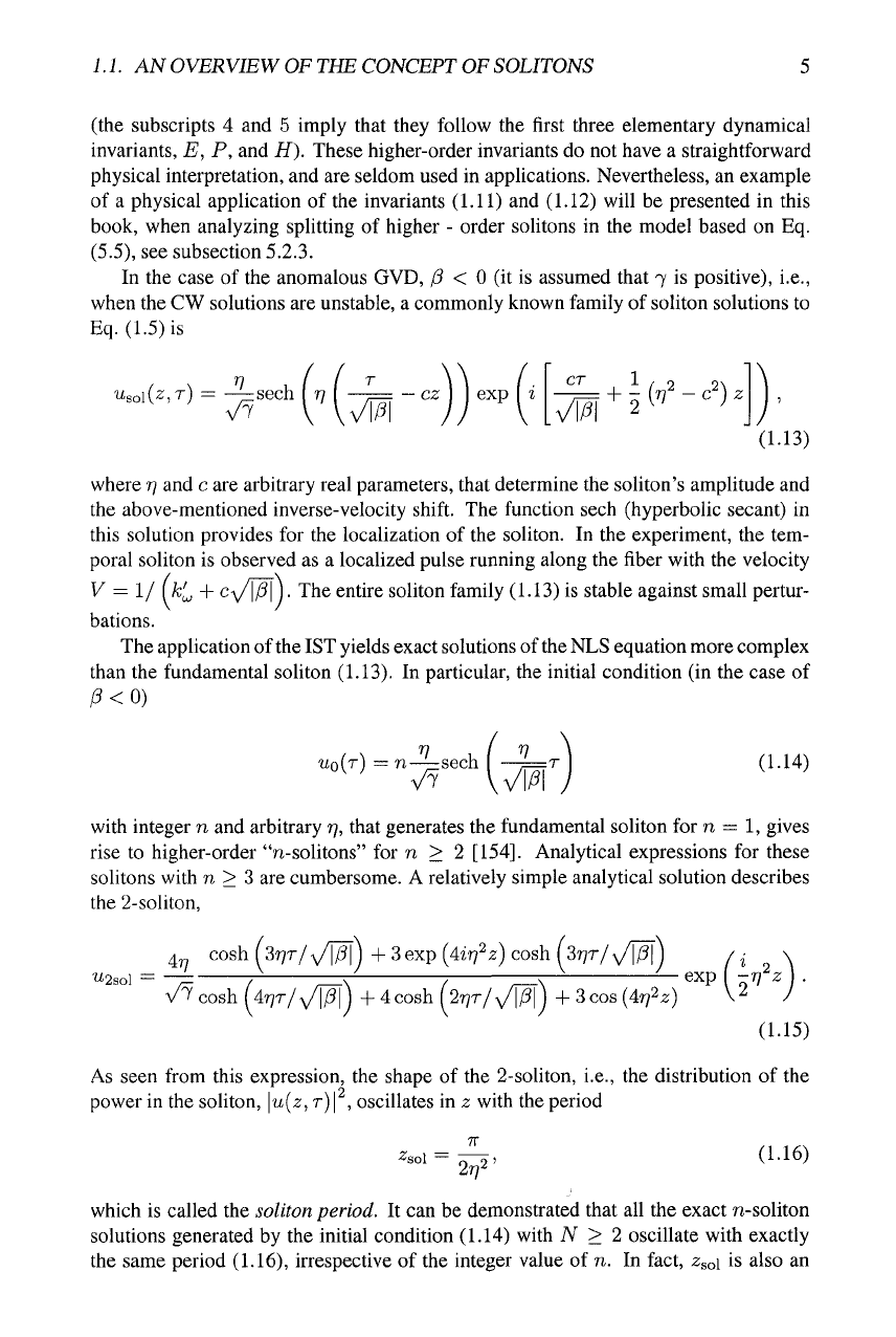
In the case of the anomalous GVD, /? < 0 (it is assumed that 7 is positive), i.e.,

when the CW solutions are unstable, a commonly known family of soliton solutions to

Eq. (1.5) is

Uso\{z,r) = —sech ( rj ( —j= - cz ) | exp

" +U^'-'')

l/?l

(1.13)

where

and c are arbitrary real parameters, that determine the soliton's amplitude and

the above-mentioned inverse-velocity shift. The function sech (hyperbolic secant) in

this solution provides for the localization of the soliton. In the experiment, the tem-

poral soliton is observed as a localized pulse running along the fiber with the velocity

y = 1/ f/c^ + cy^j^

The entire soliton family (1.13) is stable against small pertur-

bations.

The application of the

1ST

yields exact solutions of the

NLS

equation more complex

than the fundamental soliton (1.13). In particular, the initial condition (in the case of

/3<0)

(1.14)

with integer n and arbitrary

rj,

that generates the fundamental soliton forn = 1, gives

rise to higher-order "n-solitons" for n > 2

[154].

Analytical expressions for these

solitons with n > 3 are cumbersome. A relatively simple analytical solution describes

the 2-soliton,

cosh

(sr^T/

VM)

exp {iirj^z) cosh (STJT/ v/pf)

U2.0I

= -p T^ —jT 7 —IT-" ^ exp -ri'z

V^ cosh

U?7T/ypl

j +

cosh

277T/\/P|

j +

cos

{irj'^z)

^ ^

(1.15)

As seen from this expression, the shape of the 2-soliton, i.e., the distribution of the

power in the soliton, \u{z,

, oscillates in z with the period

2sol=^, (1.16)

which is called the soliton

period.

It can be demonstrated that all the exact n-soliton

solutions generated by the initial condition (1.14) with N > 2 oscillate with exactly

the same period (1.16), irrespective of the integer value of n. In fact, ^soi is also an

6 INTRODUCTION

estimate for the propagation distance which is necessary for formation (self-trapping)

of the fundamental soliton from an initial pulse of a generic form.

As well as the fundamental soliton (1.13), the 2-soliton (1.15) remains single-

humped at any z (i.e., |w(2:,r)| always has a single maximum as a function of r).

However, the 3-soliton solution periodically splits into a double-humped structure and

recombines into a sharp single-peak one, see Fig. 5.4 in book [15].

In terms of the

1ST,

the 2-soliton (1.15) may be regarded as a nonlinear bound state

of two fundamental solitons, with the amplitudes

4-='^

3r,,4-='^=n.

(1.17)

Similarly, the 3-soliton is a bound state of three fundamental solitons, with

Note that the energy (1.9) of the n-soliton (1.14) is

En = ^^^^nV (1.19)

As follows from the above and Eq. (1.19), for n = 2 and n = 3 (actually, for any n)

the energy of the n-soliton is exactly equal to the sum of energies of the constituent

fundamental solitons, if they are separated from each other. To understand if the bound

state is stable against splitting into the separate fundamental solitons, one can identify

its binding potential, as a difference between the value of the Hamiltonian (1.8) for the

n-soliton, which is

Hn = ^rfv? (2n2 - l) , (1.20)

and the sum of the values of H for the separated constituent solitons. The result is

that the binding potential is exactly equal to zero for all the n-solitons. For this reason,

they are considered as unstable states. Indeed, an initial perturbation which imparts

infinitely small velocities to the constituent solitons will result in splitting. However,

this is a slowly growing instability, rather than exponential growth of perturbations,

which would imply usual dynamical instability. For this reason, n-solitons may be

physically meaningful objects.

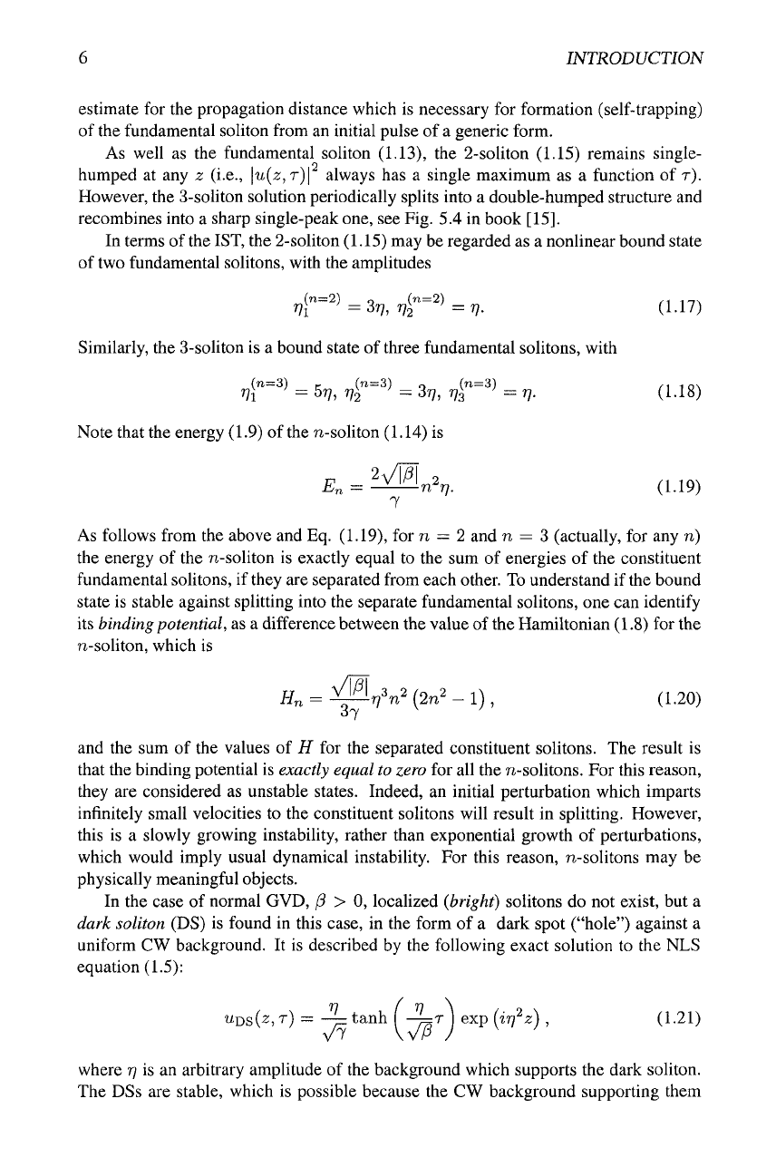
In the case of normal GVD, /9 > 0, localized {bright) solitons do not exist, but a

dark soliton (DS) is found in this case, in the form of a dark spot ("hole") against a

uniform CW background. It is described by the following exact solution to the NLS

equation (1.5):

I n \

ur)s(.z,T) = -—tanh ( -J^TJ exp (ir/^z), (1.21)

where

is an arbitrary amplitude of the background which supports the dark soliton.

The DSs are stable, which is possible because the CW background supporting them

1.1.

AN OVERVIEW OF THE CONCEPT OF SOLITONS

is itself modulationally stable for /3

0, as mentioned above. DSs were created ex-

perimentally in nonlinear optical fibers [60, 98, 172], about a decade after the first

observation of the bright solitons in fibers was reported. DSs are not a subject of this

book, except for a brief consideration in the context of the ID Feshbach-resonance-

driven Bose-Einstein condensate, see

Fig.

5.3 and related text. A review of DSs can be

found in article [91].

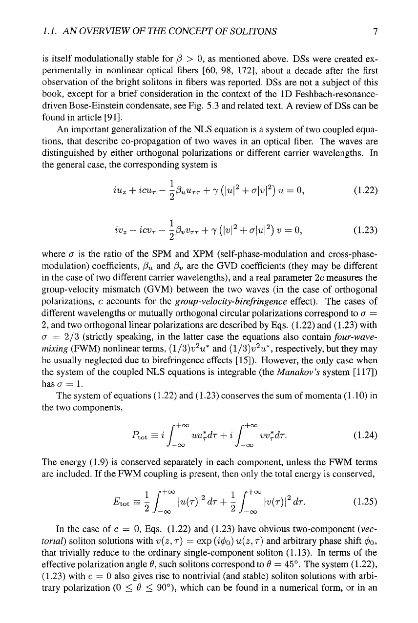
An important generalization of the NLS equation is a system of two coupled equa-

tions,

that describe co-propagation of two waves in an optical fiber. The waves are

distinguished by either orthogonal polarizations or different carrier wavelengths.

the general case, the corresponding system is

iu^

+ icur

-PUUTT

+ 7 {\u\^ + cr|t;|^)

0, (1.22)

iv^

icVr

-pvVrr

+ 7

(^P

<^H'^)

=0,

(1.23)

where

is the ratio of the SPM and XPM (self-phase-modulation and cross-phase-

modulation) coefficients, /?„ and fiy are the GVD coefficients (they may be different

in the case of two different carrier wavelengths), and a real parameter 2c measures the

group-velocity mismatch (GVM) between the two waves (in the case of orthogonal

polarizations, c accounts for the gwup-velocity-birefringence effect). The cases of

different wavelengths or mutually orthogonal circular polarizations correspond to

a =

and two orthogonal linear polarizations are described by

Eqs.

(1.22) and (1.23) with

2/3 (strictly speaking, in the latter case the equations also contain/owr-wave-

mixing (FWM) nonlinear terms,

{l/2>)v'^u*

and (1/3)I)^M*, respectively, but they may

be usually neglected due to birefringence effects [15]). However, the only case when

the system of the coupled NLS equations is integrable (the Manakov's system [117])

has

The system of equations (1.22) and (1.23) conserves the sum of momenta (1.10) in

the two components,

Ptot =«

uu*^dT

+ i

vv*dT.

(1-24)

The energy (1.9) is conserved separately in each component, unless the FWM terms

are included. If the FWM coupling is present, then only the total energy is conserved,

Etot^^j_

\u{TfdT+-J^ \v{T)fdT.

(1.25)

In the case of c

0, Eqs. (1.22) and (1.23) have obvious two-component (vec-

torial) soliton solutions with v{z, r)

exp (i(/io) u{z, r) and arbitrary phase shift

(t)o,

that trivially reduce to the ordinary single-component soliton (1.13). In terms of the

effective polarization angle 9, such solitons correspond to 9

—

45°. The system (1.22),

(1.23) with c

0 also gives rise to nontrivial (and stable) soliton solutions with arbi-

trary polarization (0 <

< 90°), which can be found in a numerical form, or in an

8 INTRODUCTION

analytical approximation by means of the VA [87] (only in the Manakov's case, a = 1,

the vectorial-soliton solutions with 9 ^ 45° can be found in an exact analytical form,

with v{z, T) = exp (j(^o) (tan

u{z,

T)).

In the spatial domain, the analysis which leads to solitons is simpler. In this case,

relevant solutions to Eq. (1.1) are looked for in the form (1.2), where the amplitude

u{z,x) may be a slowly varying function of z and the transverse coordinate x, while

the time delay in e is irrelevant, i.e., e =

CQ-

The latter implies setting

= feo/^/eo in

the expression for the carrier wave in Eq. (1.2), then the first nontrivial approximation

leads to the following nonlinear equation for the slowly varying amplitude,

iu^

+ -—-u^x+-i\u\^u =

(1.26)

where the relation / =

|M|^

is again taken into regard, and this time the nonlinearity

coefficient is defined as 7 = n2ko/y/eo. The spatial-domain equation (1.26) takes ex-

actly the same form (with the same relative signs in front of the second derivative and

nonlinear term) as the NLS equation (1.5) in the temporal domain with the anomalous

GVD (i.e., the transverse diffraction in the spatial domain is a counterpart to the nega-

tive GVD in the temporal domain). Accordingly, the family of solutions (1.13), with T

replaced by x, describes spatial solitons, in the form of localized planar beams of light

in the two-dimensional plane (z, x). The solutions with c ^ 0 correspond to the beams

tilted relative to the z axis.

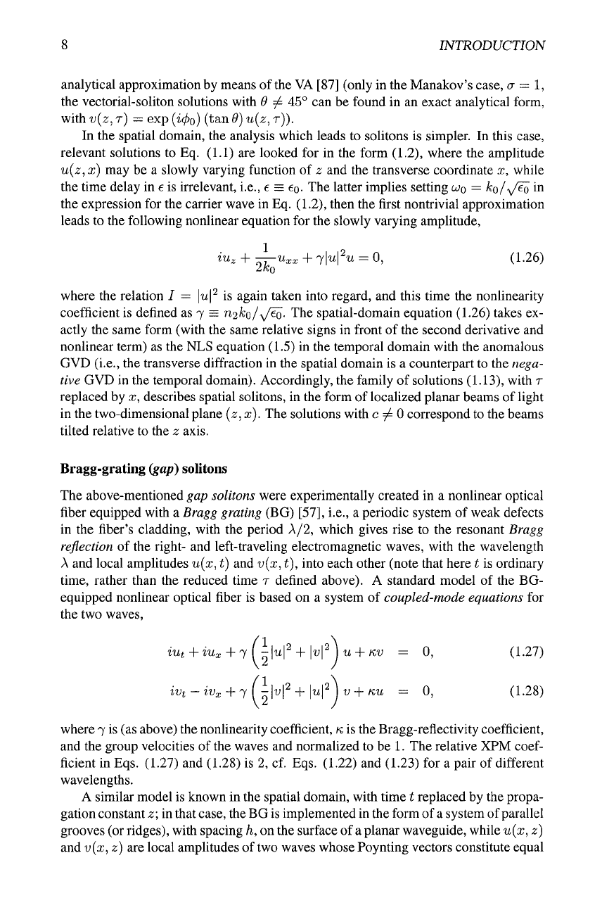
Bragg-grating (gap) solitons

The above-mentioned gap solitons were experimentally created in a nonlinear optical

fiber equipped with a Bragg grating (BG) [57], i.e., a periodic system of weak defects

in the fiber's cladding, with the period A/2, which gives rise to the resonant Bragg

reflection of the right- and left-traveling electromagnetic waves, with the wavelength

and local amplitudes u{x, t) and v{x, t), into each other (note that here t is ordinary

time,

rather than the reduced time T defined above). A standard model of the BG-

equipped nonlinear optical fiber is based on a system of coupled-mode equations for

the two waves,

iut + iU:,+-i\--\uY + \vY\u +

= 0, (1.27)

ivt-ivx+^

{-\vY •\-\uY\v +Ku = 0, (1.28)

where 7 is (as above) the nonlinearity coefficient,

is the Bragg-reflectivity coefficient,

and the group velocities of the waves and normalized to be 1. The relative XPM

coef-

ficient in Eqs. (1.27) and (1.28) is 2, cf. Eqs. (1.22) and (1.23) for a pair of different

wavelengths.

A similar model is known in the spatial domain, with time t replaced by the propa-

gation constant z; in that

case,

the BG is implemented in the form of

system of parallel

grooves (or ridges), with spacing h, on the surface of

planar waveguide, while u{x,z)

and ti(x, z) are local amplitudes of two waves whose Poynting vectors constitute equal