Malomed B.A. Soliton Management in Periodic Systems
Подождите немного. Документ загружается.

2.2.
THE MODEL WITH THE HARMONIC MODULATION
29
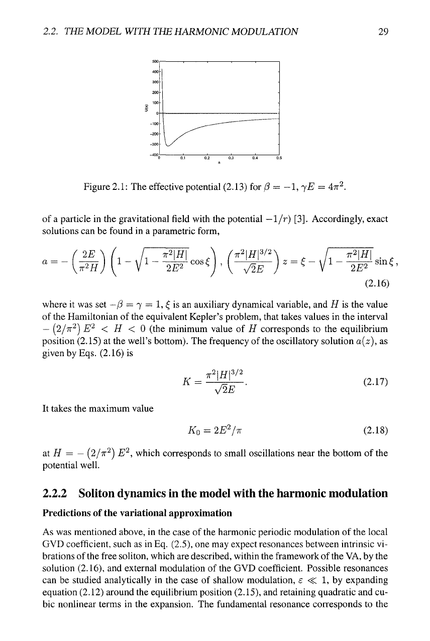
Figure
2.1:
The effective potential (2.13) for p = -1, jE =
ATT"^
of a particle in the gravitational field with the potential — 1/r) [3]. Accordingly, exact
solutions can be found in a parametric form,
cos^
7r^|g|3/2
V2E
z
= e-
TT^\H\
2^2
sinC,
(2.16)
where it was set
—f3
= 7 = 1, ^ is an auxiliary dynamical variable, and H is the value
of the Hamiltonian of the equivalent Kepler's problem, that takes values in the interval
—
(S/TT^) E^ < H < 0 (the minimum value of H corresponds to the equilibrium
position (2.15) at the well's bottom). The frequency of the oscillatory solution a(z), as
given by Eqs. (2.16) is
K =
,2|_ff|3/2
V2E
It takes the maximum value
Ko =
2E^/TT
(2.17)
(2.18)
&l
H = - (2/7r2)
E"^,
which corresponds to small oscillations near the bottom of the
potential well.
2.2.2 Soliton dynamics in the model with the harmonic modulation
Predictions of tlie variational approximation
As was mentioned above, in the case of the harmonic periodic modulation of the local
GVD coefficient, such as in Eq. (2.5), one may expect resonances between intrinsic vi-
brations of the free soliton, which are described, within the framework of
the
VA,
by the
solution (2.16), and external modulation of the GVD coefficient. Possible resonances
can be studied analytically in the case of shallow modulation, e -C 1, by expanding
equation (2.12) around the equilibrium position (2.15), and retaining quadratic and cu-
bic nonlinear terms in the expansion. The fundamental resonance corresponds to the
30
DISPERSION MANAGEMENT
case when the (spatial) frequency KQ of free small oscillations near the equilibrium
position, given by Eq. (2.18), is close to the spatial modulation frequency, which is 1
in Eq. (2.5). In other words, varying the initial soliton's energy E, one may expect that
the fundamental resonance occurs in a vicinity of the value -Efundam = \/7r/2 » 1.25.
Further, the first subharmonic resonance, corresponding to 2Ko close to 1, and the
second-order resonance, which takes place for KQ close to 2, are expected around
^subharm = \/7r/2 « 0.87 and £^second = \/7r » 1.77, respectively.
Actual predictions of the VA should be obtained by from numerical simulations of
Eq. ((2.12) with (i{z) =
—
(1 + esinz). In particular, a solution with a{z) ^ c» at
2;
—+
oo is interpreted as destruction of the soliton, as it becomes infinitely broad. In
fact, this implies decay of the soliton into radiation.
The simulations performed in work [110] have demonstrated that, in an interval of
values of the soliton's energies E which covers both the above-mentioned first sub-
harmonic and second-order resonances, oscillations of a{z) driven by the sinusoidal
modulation of ^{z) are anharmonic but still periodic at very small values of e, typi-
cally £ ~ 0.01. With the increase of the modulation depth e, the oscillations become
nonperiodic at £ ~ 0.05, and apparently chaotic at £ closer to 0.20. Finally, a criti-
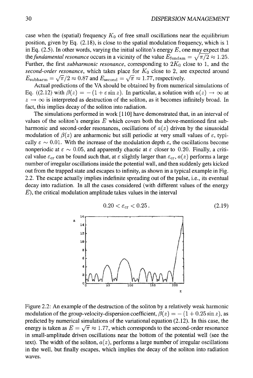
cal value £cr can be found such that, at e slightly larger than £cr, a{z) performs a large
number of irregular oscillations inside the potential wall, and then suddenly gets kicked
out from the trapped state and escapes to infinity, as shown in a typical example in Fig.
2.2.
The escape actually implies indefinite spreading out of the pulse, i.e., its eventual
decay into radiation. In all the cases considered (with different values of the energy
E),
the critical modulation amplitude takes values in the interval
0.20 <£cr <0.25.
(2.19)
Figure 2.2: An example of the destruction of the soliton by a relatively weak harmonic
modulation of the group-velocity-dispersion coefficient, P{z) =
—
(1 + 0.25 sin z), as
predicted by numerical simulations of the variational equation (2.12). In this case, the
energy is taken as E = yjii « 1.77, which corresponds to the second-order resonance
in small-amplitude driven oscillations near the bottom of the potential well (see the
text).
The width of the soliton, a{z), performs a large number of irregular oscillations
in the well, but finally escapes, which implies the decay of the soliton into radiation
waves.
2.2.
THE MODEL WITH THE HARMONIC MODULATION
31
In the case when the modulation amplitude £
is
small, the rate
of
direct emission
of radiation by the soliton (obviously, this effect is beyond the scope of the VA) can be
calculated by means of the perturbation theory [4]; however, this process does not play
a crucial role in the destruction of the soliton.
Numerical results
The predictions produced by VA for the soliton in the NLS equation (2.5) with the si-
nusoidally modulated local GVD were compared with results
of
direct simulations of
the equation in work [76]. Results of the simulations are summarized in Fig. 2.3. Two
gross feature
of
this diagram roughly comply with predictions
of
the VA. Firstly, the
destruction of the soliton may take place if the modulation amplitude exceeds a critical
value, which varies, essentially, within an interval 0.15
<
Sa <
0.20, that should be
compared to interval (2.19) predicted by VA. Secondly, the destruction
of
the soliton
actually takes place, for
e
not too large,
if
the initial squared soliton's energy E'^ ex-
ceeds
a
minimum value E^^^ varying between 1.8 and 2.0, which may be compared
to the above-mentioned value -E^undam
=
^/2 that gives rise to the fundamental reso-
nance between small vibrations of the perturbed soliton and the periodic modulation of
the local GVD in Eq. (2.5).
• ••
U
Boao
0D D D
ania
• D D D
B D D D
Dfiio
PfOB
nanf
DHPQ
nnaa
OBDQ
pasn
Hid
D
ID30
•GlaoD
• aaa
30
a fi D Q o n
n a n n a D
Maaaac
oaDaoc
Sa a a d c
• • • •
a
c
naanac
G u u u uQ
D D D D DO
D D•aaa
noOBIIB
&iBDaB
D [3 D D
DODD
n DO"
•
aan
•
BBC
• Buu
BBina
Bn • •
Bono
• oca
gnnn
•3 •••
a 3 o D D
go n CL C •
p a D D D n
3 a 3 c- • D
•O3C0D
•3
C
3
C
Q
ta
a
c
J
c
•
3
a
c
3
a a
[1
a
c
3
n n
anu no
a u.
=]«•
poiaa
i::3s
DaannBROSDaaBiiQaBiiB
Figure
2.3:
The phase diagram in the parametric plane i£,E^) for solitons in Eq. (2.5).
The filled and unfilled rectangles correspond, respectively, to stable and splitting soli-
tons.
The most essential difference between the assumptions on which the VA was based
and numerical results is that the fundamental mode of the soliton destruction under the
action of the sinusoidally modulated dispersion is not decay into radiation, but splitting
of the soliton into two apparently stable secondary solitons (which is accompanied by
emission
of a
considerable amount
of
radiation).
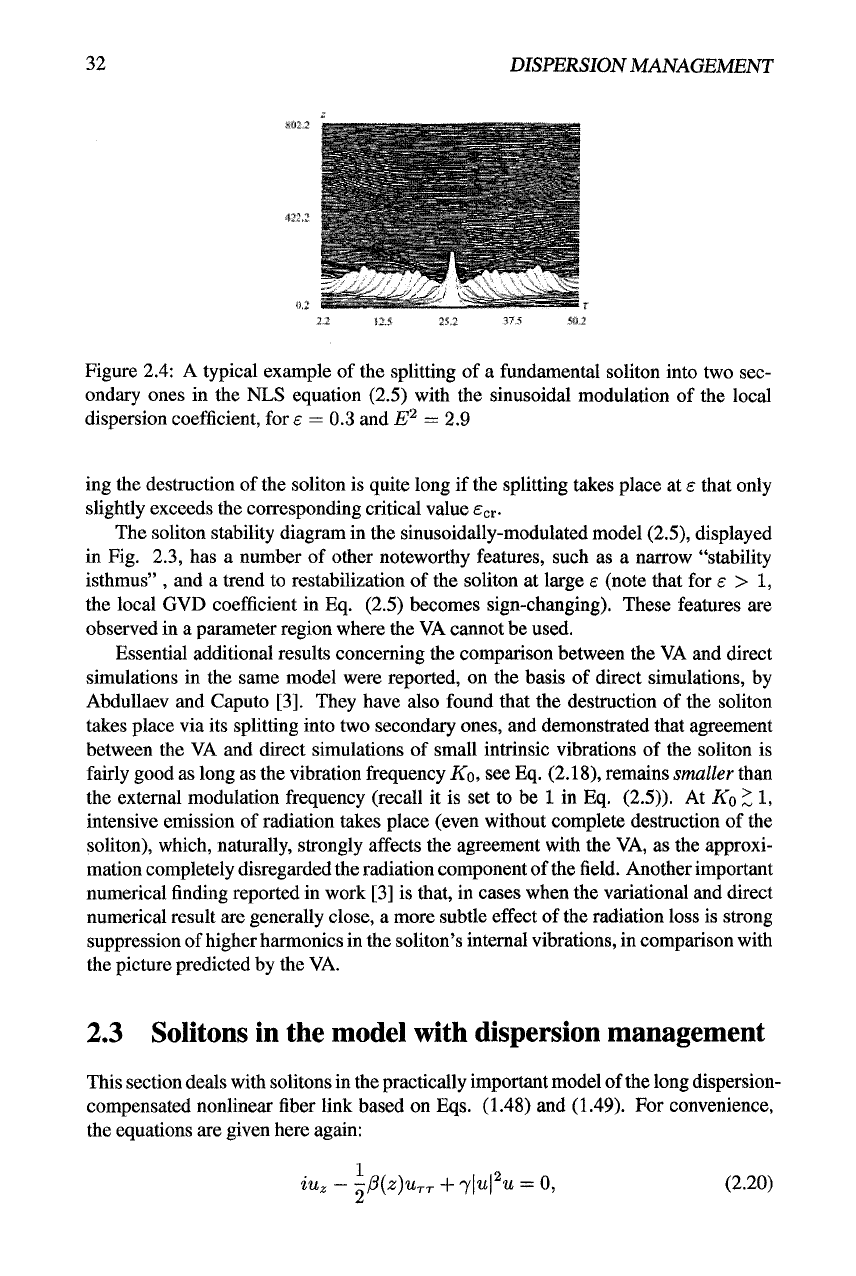
A
typical example
of
the splitting
in displayed
in
Fig.
2.4.
Obviously, the ansatz (2.6) does not admit any splitting;
nevertheless, basic characteristics
of
the destruction
of
the soliton, even
if
the actual
destructions mode is different from the one postulated by the VA, are predicted by the
approximation qualitatively and semi-quantitatively correctly.
Detailed inspection
of
the numerical results shows that, prior to the splitting, the
soliton performs
a
number
of
irregular vibrations, which resembles the picture pro-
duced by the VA, cf. Fig. 2.2. As well as in that picture, the vibrational stage preced-
32 DISPERSION MANAGEMENT
^i^^^^^^fi:^
•^mmm
^^<
3.2
12.5 2S.2 37.5 SOI
Figure 2.4: A typical example of the splitting of a fundamental soliton into two sec-
ondary ones in the NLS equation (2.5) with the sinusoidal modulation of the local
dispersion coefficient, for e
=
0.3 and
E'^
=
2.9
ing the destruction of the soliton is quite long if the splitting takes place at e that only
slightly exceeds the corresponding critical value ecr-
The soliton stability diagram in the sinusoidally-modulated model (2.5), displayed
in Fig. 2.3, has a number of other noteworthy features, such as a narrow "stability
isthmus"
,
and a trend to restabilization of the soliton at large e (note that for e
> 1,
the local GVD coefficient in Eq. (2.5) becomes sign-changing). These features are
observed in a parameter region where the VA cannot be used.
Essential additional results concerning the comparison between the VA and direct
simulations in the same model were reported, on the basis of direct simulations, by
Abdullaev and Caputo [3]. They have also found that the destruction of the soliton
takes place via its splitting into two secondary ones, and demonstrated that agreement
between the VA and direct simulations of small intrinsic vibrations of the soliton is
fairly good as long as the vibration frequency Ko, see Eq. (2.18), remains smaller than
the external modulation frequency (recall it is set to be 1 in Eq. (2.5)). At ii'o ^ 1,
intensive emission of radiation takes place (even without complete destruction of the
soliton), which, naturally, strongly affects the agreement with the VA, as the approxi-
mation completely disregarded
the
radiation component of the field. Another important
numerical finding reported in work [3] is that, in cases when the variational and direct
numerical result are generally close, a more subtle effect of the radiation loss is strong
suppression of higher harmonics in the soliton's internal vibrations, in comparison with
the picture predicted by the VA.
2.3 Solitons in the model with dispersion management
This section deals with solitons in the practically important model of the long dispersion-
compensated nonlinear fiber link based on Eqs. (1.48) and (1.49). For convenience,
the equations are given here again:
iu,
-
-p{z)urT +
y\u\'^u
=
0, (2.20)
2.3.
SOLITONS IN THE MODEL WITH DISPERSION MANAGEMENT 33
r /?i >0, if 0<z<Li,
^ ~ \ /32 < 0, if L,<z<Li+L2 = L, ^^•^^'
The concept of
the
dispersion management (DM) for solitons in dispersion-compensated
systems which, in the simplest case, amount to the model based on Eqs. (2.20) and
(2.21),
was introduced nearly simultaneously in works by Knox, Forysiak, and Do-
ran [95], Suzuki, Morita, Edagawa, Yamamoto, Taga, and Akiba
[160],
Nakazawa and
Kubota
[131],
and Gabitov and Turitsyn [69]. The original motivation for the develop-
ment of the DM technique for solitons was the necessity to suppress the Gordon-Haus
effect, i.e., random jitter of the soliton's center due to its interaction with optical noise,
which is accumulated in the fiber-optic link due to the spontaneous emission from the
optical amplifiers (these are actually Erbium-doped segments of the fiber, periodically
inserted into the link, with the objective to compensate the fiber loss). The dispersion-
managed solitons were predicted (and found in the experiment) to have large energy,
which helps to improve the noise-to-signal ratio. Indeed, it has been demonstrated
that the DM technique is very efficient in stabilizing solitons against the random jit-
ter. On the other hand, a problem for the use of solitons in the DM system is posed
by interactions between them. As the DM solitons periodically expand and contract,
they may tangibly overlap, through their "tails", at the expansion stage, which leads to
the increase of unwanted interaction between them. Besides their great significance to
the applications, solitons in DM models have also drawn a great deal of attention as a
subject of fundamental research. The account given below focuses chiefly on the latter
point, although applied aspects are briefly considered too.
As explained below, the VA is a very natural tool to investigate the soliton dynam-
ics in DM models. The presentation in this section will chiefly follow the approach
elaborated in works [100] and [106] (the latter work applied the VA, in combination
with direct simulations, to solitons in a model of random DM). In particular, the same
normalization of parameters of the DM map (2.21) as in paper [100] is adopted here,
(/3i - /3o) Li + (/32 - /3o) L2 = 0, lA " /3o|ii = |/32 - /3o|L2 = 1, L = Li -f- L2 = 1,
(2.22)
which can be always imposed by means of an obvious rescaling (recall /3o is the PAD
defined as per Eq. (1.50)).
In the case of strong DM, when the nonlinear term in Eq. (2.20) may be treated as
a small perturbation, the RZ Gaussian pulse (1.51), which is the exact solution in the
linear limit, may be used as a natural variational ansatz, to take into regard effects of
the weak nonlinearity. For convenience, the ansatz is written here again:
"^^("'^) = ^/^
.
2i5(.)/>yo2 exp (-^ - ^^j^^ , (2.23)
B{z) = Bo+ [ (3{z')dz' (2.24)
Jo
The PAD will also be treated as a small perturbation, as an intuitive assumption
is that the weak nonlinearity and small PAD may effectively compensate each other,
34 DISPERSION MANAGEMENT
supporting a robust RZ pulse (alias, DM soliton). An important dimensionless char-
acteristic of the pulse (2.23) is its dispersion-management strength, which is defined
as
5^1443Nia + |^^_ (2.25)
The factor 1.443 appears here due to the use of the so-called FWHM (full-width-at-
half-maximum) definition of the pulse's width, which is different from
WQ.
According
to the value of S, the DM schemes are usually categorized as
weak-DM,
moderate-
DM, and strong-DM regimes - in the cases of, roughly, 5 < 3, 5 ~ 3
—
4, and S > A,
respectively.
The VA is based on the assumption that the arbitrary constants
WQ
and
BQ
in Eqs.
(2.23) and (2.24) become slowly varying functions of z, if the weak nonlinearity is
taken into regard. Additionally, the accumulated dispersion B{z) is defined for the
map (2.21) from which the PAD value /3o is subtracted. The analysis presented in
detail in paper [100] yields the following evolution equations for the slowly varying
parameters:
dW,
j^EWoB{z)
dB^^
E^izy-W^
(2.27)
dz
^°
2V2W^z)
where the function W{z) is defined in Eq. (1.53). To derive these equations, the nor-
malization (2.22) was used, and the energy of the pulse is defined
&s
E —
PQTO
(recall
that
PQ
is peak power, i.e., maximum value of the squared amplitude, in expression
(2.23)).
In fact, E plays the role of a small parameter measuring the relative weakness
of the nonlinearity in comparison with the local dispersion.
An issue of fundamental interest is to find conditions allowing for the stationary
transmission of the pulse, i.e., a dynamical regime in which the parameters
WQ
and
BQ
return to their initial values after passing one DM period. Because, as it is seen from
Eqs.
(2.26) and (2.27), changes of Wo and BQ within one period are generally small,
~ (/3o, E), in the first approximation one may insert unperturbed values of WQ and
BO
into the right-hand sides of
Eqs.
(2.26) and (2.27), and impose the conditions that
(recall that the DM period is 1 in the present notation)
'''^Uz=r'-^dz
= 0. (2.28)
dz
Jo dz
After some analytical calculations,
Eqs.
(2.28) yield the following stationary-propagation
conditions for the Gaussian pulse in an explicit form,
Bo =
-^
,
1^0
= "^-^'^0
VW+^
(2.29)
2.3.
SOLITONS IN THE MODEL WITH DISPERSION MANAGEMENT 35
The meaning of the condition
BQ
= 1/2 is quite simple: it requires the pulse to
have zero chirp at the midpoint of each fiber segment. The second condition (2.29)
predicts that the DM soliton propagates steadily at anomalous PAD, /?o < 0, provided
that W^ >
(W^)^^
« 0.30, at
/3o
= 0 if Wg =
(W^)^,,
and at normal PAD, po > 0,
if (W^o^)jjii„ » 0.148 < W^ <
(W^)^^.
The latter case is very interesting, as the
classical NLS soliton cannot exist at normal dispersion. Further analysis of
Eq.
(2.29)
shows that, in this case, the solution exists in a limited interval of the normal-PAD
values,
0 < f3o/E < iPo/E)^^^ « 0.0127. (2.30)
Inside this interval, Eq. (2.29) yields two different values of the minimum width
Wo for a given value of (3o/E, while in the anomalous-PAD region,
WQ
is a uniquely
defined function of f3o/E. In the case of the normal PAD, /?o > 0, it can be concluded
that the DM soliton corresponding to the larger value of
WQ
is stable, while the one
corresponding to smaller
WQ
is unstable. The border between the stable and unstable
solitons corresponds to (3o/E = {Po/E)^^^ (see Eq. (2.30)), and it is located at
WQ
= {WQ) • ~ 0.148 (i.e., all the stable and unstable solitons have, respectively,
W^ > (Wg^)^.^ and
WQ^
<
{W^)^.^J.
The results concerning the stability of these
two solitons were substantiated in a mathematically rigorous form in work
[140].
Translating
WQ
into the standard DM-strength parameter 5 according to
Eq.
(2.25),
one concludes that the VA predicts the following:
•
•
stable DM solitons at anomalous PAD if 5 < Scr ~ 4.79;
• stable DM solitons at zero PAD if 5 = 5cr « 4.79;
stable DM solitons at normal PAD if 4.79 < S < 5max » 9.75;
• no stable DM soliton for S > S^ax ~ 9.75.
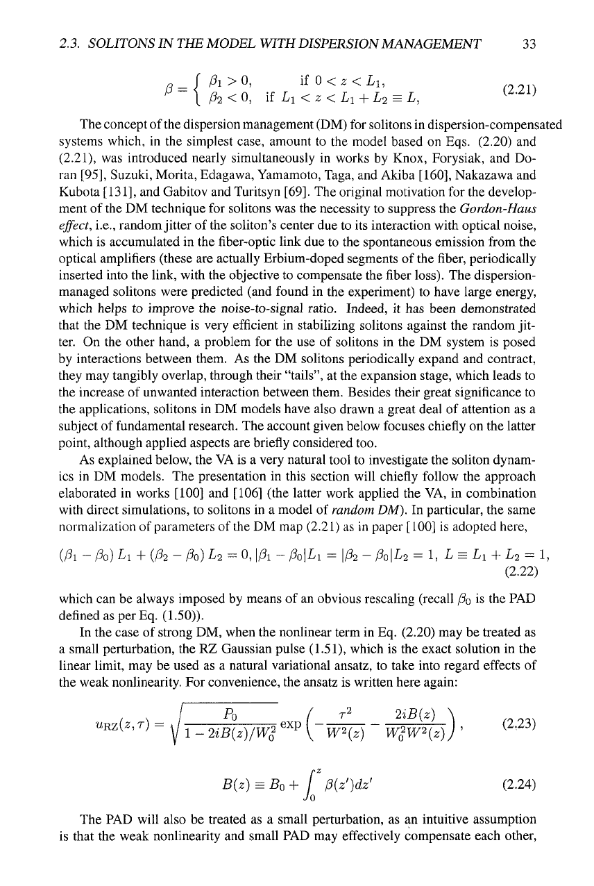
The normalized power of the DM soliton, which is P = 4 •
1.12Po
(the factor
1.12 is the ratio of the FWHM widths for the sech-shaped and Gaussian pulses) is
shown vs. the DM strength, at several fixed values of PAD /3o, as predicted by Eq.
(2.29),
in Fig. 2.5. A counterpart of the same dependence, obtained in work [31] from
direct simulations of the underlying equation (2.20), is displayed in Fig. 2.6 (a typical
example of the shape of the DM soliton, found from direct simulations, is displayed
below in Fig. 2.10). In Fig. 2.5, the curves are shown only in the region of 5 < 9.75,
where the solitons are expected to be stable. The curves in Fig. 2.6 corresponding
to the normal PAD (/3o > 0) terminate at points where the corresponding DM soliton
becomes unstable.
As a matter of fact, Fig. 2.6 is the most fundamental and comprehensive character-
istic of the family of the DM solitons. The comparison of
Figs.
2.5 and 2.6 shows that
the
VA
yields acceptable results for relatively small values of
the
soliton's power, where
the underlying assumption, that the nonlinearity may be treated as a weak perturbation,
is relevant. In particular, the VA-predicted critical value Scr » 4.79 is different from
but nevertheless reasonably close to the critical DM strength ^cr « 4 which direct sim-
ulations yield in the small-power limit. With the increase of power, numerically found
36 DISPERSION MANAGEMENT
E"
* / ^r \
P
-0.02 / _
°/ P„-0
T""^
,
, )t, . . , ,
Map stcength, S
Figure
2.5:
The peak power of the stable soliton in the DM system vs. the map strength
S at different values of the path-average dispersion
/3o,
as predicted by the variational
approximation based on Eq. (2.29). Here and in the next figure, stars mark cases for
which the corresponding model with random DM was investigated in detail, see section
2.4.
..
I:
'
h
-0,2
fh'O
(io-0.02
P^=0.02
Map strength, S
Figure 2.6: A counterpart of Fig. 2.5 obtained from direct numerical simulations of
Eq. (2,20).
S'cr grows. It is also noteworthy that the value ^max ^ 9-75, predicted by the VA as
the stability limit for the DM solitons, is indeed close to what is revealed by direct
simulations for small powers, as seen in Fig. 2.6.
The DM soliton considered above is a fundamental one (i.e., it always keeps the
single-peak shape). Higher-order DM solitons can be constructed too. Indeed, along
with the expression (2.23), its r-derivatives of all orders are also exact solutions to the
linearized version of Eq. (2.20), and can be used as ansdtze to generate an (approx-
imate) higher-order soliton solutions in the weakly nonlinear case. In particular, an
ansatz proportional to the first derivative of the Gaussian (2.23),
(«([r^)(.,r))^
Po
dd Y
1
-
2iB{z)IW^
W^z)
exp
r^ 2iB{z)
'W^z)~W^Vr\z
(2.31)
was used in work [137] to construct an odd (antisymmetric, as a function of r) DM
soliton. However, this soliton is unstable against even perturbations. Related to this
2.4. RANDOM DISPERSION MANAGEMENT 37
generalization is another technical approach to the description of the fundamental DM
solitons and perturbations around them: an extended solution, including the perturba-
tion, may be looked for starting from a linear combination of Hermite-Gauss functions
(of r) [167, 99]. In particular, this approach correctly reproduces the results of the VA.
2.4 Random dispersion management
Existing terrestrial fiber-optic telecommunication networks are patchwork systems,
which include links with very different lengths [16]. This practically important cir-
cumstance suggests to consider transmission of RZ pulses (quasi-solitons) in random
DM systems. It was shown that VA applies to this case too
[106].
Random-DM mod-
els of different types were considered in works [1] and [73], where local values of the
GVD coefficient, rather than the fiber-segment lengths, are distributed randomly. Ac-
tually, search for robust RZ pulses in random nonlinear fiber-optic systems is an issue
not only important to the applications, but also fundamentally significant to the general
theory of nonlinear waves in disordered media [96].
The basic equation and normalizations for the DM system with random distribution
of the cell lengths can be taken in the same form as in the previous section, i.e., as per
Eqs.
(2.20), (2.21), and (2.22), with a difference that, in the random system, the nor-
malizations must be applied to mean values of the randomly varying lengths. The con-
sideration is limited here to the most important case when the lengths of the segments
with the anomalous and normal GVD are equal in each DM cell, Li = L2 ^ L/2.
Then, Eqs. (2.22) yield the mean values Li,2 = 1/2, and |/3i,2
—
Po\
=2. To com-
ply with the former condition, one may assume that the random lengths are distributed
uniformly in the interval
0.1<L/2<0.9. (2.32)
The minimum length 0.1 is introduced because, in reality, the length can be neither
very large (say, larger than 200 km) nor very small (shorter than 20 km).
The same ansatz (2.23) and variational equations (2.26) and (2.27) which was ap-
plied above to the regular (periodic) DM system, may be used with its random coun-
terpart. As explained above, the change of the soliton's parameters,
WQ
—>
WQ
+ 5Wo,
Bo
—^
Bo + SBo, within one DM cell is small. Therefore, the evolution of the pulse
passing many cells may be approximated by smoothed differential equations,
dWo _ 5Wo dBo _ 5Bo
dz L(") ' dz L(") ^ '
38
DISPERSION MANAGEMENT
(n is the cell's number). Finally, the equations take the following form,
dWo
dz
dBo
dz
\/W^o+4Bo^ ^W^ + ^{B^-L{z)y
(2.34)
Pa
^/2EW^
4Bo
4(-Bo-L)
8L(z) [^W^ + AB- ^W^ + A{B,-L{z)f
+ ln
^W^ + ABl - 2Bo
^
^W^ + 4 (Bo - L{z)f -2 {Bo- Liz))
^
(2.35)
where L{z) is regarded as a continuous random function with values uniformly dis-
tributed in the interval (2.32).
The most essential characteristic of the pulse propagation at given values of
/3o
and
E is the cell-average pulse's width,
W
W{z)dz.
(2.36)
cell
Simulations of
Eqs.
(2.34) and (2.35) reveal that there are two drastically different dy-
namical regimes. If the soliton's energy is sufficiently small (hence the approximation
outlined in the previous section is relevant) and PAD is anomalous or zero, i.e.,
/3o
< 0
(especially, if
/?o
= 0), the pulse performs random vibrations but remains truly stable
over long propagation distances. In the case when the energy is larger, as well as when
PAD is normal,
/3o
> 0, the pulse suffers fast degradation.
Following work
[106],
typical examples of the propagation are displayed in Fig.
2.7 for the zero-PAD case, which is the best one in terms of the soliton stability. Sim-
ulations of Eqs. (2.34) and (2.35) were performed with 200 different realizations of
the random function L{z). Figure 2.7 displays the evolution of {W{z)), i.e., mean
value of the width (2.36) averaged over the 200 random realizations, along with the
corresponding normal deviations from the mean value. The figure demonstrates that
some systematic slow evolution takes place on top of the random vibrations, which are
eliminated by averaging over 200 realizations. Systematic degradation (broadening) of
the soliton takes place too, but it is extremely slow if the energy is small. In the case
shown in the bottom part of Fig. 2.7, the pulse survives, with very little degradation,
the transmission through more than 1000 average cell lengths (in fact, as long as the
simulations could be run). It is not difficult to understand this: in the limit of zero
power, i.e., in the linear random-DM model, an exact solution for the pulse is available
in an essentially the same form as given above for the periodic DM, see Eq. (2.23). If
PAD is exactly zero, this exact solution predicts no systematic broadening of the pulse.
If the soliton's energy is larger, further simulations of
Eqs.
(2.34) and (2.35) show
that, after having passed a very large distance, the slow spreading out of the soliton
suddenly ends up with its blowup (complete decay into radiation). This seems to be
qualitatively similar to what was predicted by the VA in the case of the periodic sinu-
soidal modulation of the dispersion, as shown in Fig. 2.2: a long sequence of chaotic