Lin S.D. Water and Wastewater Calculations Manual

Подождите немного. Документ загружается.

Using Eq. (3.16)

⫽ 2 ⫻ 3.14 ⫻ 0.00134 m/s ⫻ 16.5 m ⫻ (35.3 –10) m/ln(264/0.46)

⫽ 0.553 m

or ⫽ 8765 gpm

2.7 Speciﬁc capacity

The permeability can be roughly estimated by a simple field well test. The

difference between the static water level prior to any pumping and the

level to which the water drops during pumping is called drawdown

(Fig. 3.2). The discharge (pumping) rate divided by the drawdown is the

specific capacity. The specific capacity gives the quantity of water produced

from the well per unit depth (ft or m) of drawdown. It is calculated by

Specific capacity ⫽ Q/wd (3.19)

where Q ⫽ discharge rate, gpm or m

wd ⫽ well drawdown, ft or m

Example: The static water elevation is at 572 ft (174.3 m) before pumping.

After a prolonged normal well pumping rate of 120 gpm (7.6 L/s), the water

level is at 564 ft (171.9 m). Calculate the specific capacity of the well.

solution:

Specific capacity ⫽ Q/wd ⫽ 120 gpm/(572 – 564)ft

⫽ 15 gpm/ft

or Specific capacity ⫽ (7.6 L/s)/(174.3 – 171.9)m

⫽ 3.17 L/s ⭈ m

3 Steady Flows in Aquifers

Referring to Fig. 3.3, if z

⫽ z

, for an unconfined aquifer,

Q ⫽ KAdh/dL (3.20)

and let the unit width flow be q, then

q ⫽ Khdh/dL

qdL ⫽ Khdh

(3.21)

Q 5 2pKm

H 2 h

ln sr/r

Groundwater 195

By integration:

(3.22)

This is the so-called Dupuit equation.

For a confined aquifer, it is a linear equation

(3.23)

where q ⫽ unit width flow, m

/d or ft

K ⫽ coefficient of permeability, m/d or ft/d

, h

⫽ piezometric head at locations 1 and 2, m or ft

L ⫽ length of aquifer between piezometric measurements,

m or ft

D ⫽ thickness of aquifer, m of ft

Example: Two rivers are located 1800 m (5900 ft) apart and fully penetrate

an aquifer. The water elevation of the rivers are 48.5 m (159 ft) and 45.6 m

(150 ft) above the impermeable bed. The hydraulic conductivity of the aquifer

is 0.57 m/d. Estimate the daily discharge per meter of width between the two

rivers, neglecting recharge.

solution:

This case can be considered as an unconfined aquifer:

K ⫽ 0.57 m/d

⫽ 48.5 m

⫽ 45.6 m

L ⫽ 1800 m

Using Eq. (3.22) the Dupuit equation:

⫽ 0.0432 m

q 5

Ksh

2 h

0.57 m/d[s48.5 md

2 s45.6 md

]

2 3 1800 m

q 5

KDsh

2 h

q 5

Ksh

2 h

qL 5 sK/2dsh

2 h

dL 5 K

hdh

196 Chapter 3

4 Anisotropic Aquifers

Most real geologic formations tend to have more than one direction for

the movement of water due to the nature of the material and its orien-

tation. Sometimes, a soil formation may have a hydraulic conductivity

(permeability) in the horizontal direction, K

, radically different from

that in the vertical direction, K

. This phenomenon (K

⫽ K

), is called

anisotropy. When hydraulic conductivities are the same in all direc-

tions, (K

⫽ K

), the aquifer is called isotropic. In typical alluvial deposits,

is greater than K

. For a two-layered aquifer of different hydraulic

conductivities and different thicknesses, applying Darcy’s law to hori-

zontal flow can be expressed as

(3.25)

or, in general form

(3.26)

where K

⫽ hydraulic conductivity in layer i, mm/s or fps

⫽ aquifer thickness of layer i, m or ft

For a vertical groundwater flow through two layers, let q

be the flow

per unit horizontal area in each layer. The following relationship exists:

(3.27)

Since

(dh ⫹ dh

⫽ (z

⫹ z

then

(3.28)

where K

is the hydraulic conductivity for the entire aquifer. Comparison

of Eqs. (3.27) and (3.28) yields

(3.29)

1 z

1 dh

5 a

1 z

1 dh

5 a

⌺K

⌺z

1 K

1 z

Groundwater 197

or, in general form

(3.30)

The ratios of K

to K

for alluvium are usually between 2 and 10.

5 Unsteady (Nonequilibrium) Flows

Equilibrium equations described in the previous sections usually over-

estimate hydraulic conductivity and transmissivity. In practical situa-

tions, equilibrium usually takes a long time to reach. Theis (1935)

originated the equation relations for the flow of groundwater into wells

and was then improved on by other investigators (Jacob, 1940, 1947;

Wenzel 1942; Cooper and Jacob, 1946).

Three mathematical/graphical methods are commonly used for esti-

mations of transmissivity and storativity for nonequilibrium flow con-

ditions. They are the Theis method, the Cooper and Jacob (straight-line)

method, and the distance-drawdown method.

5.1 Theis method

The nonequilibrium equation proposed by Theis (1935) for the ideal

aquifer is

(3.31)

and

(3.32)

where d ⫽ drawdown at a point in the vicinity of a well pumped

at a constant rate, ft or m

Q ⫽ discharge of the well, gpm or m

T ⫽ Transmissibility, ft

/s or m

r ⫽ distance from pumped well to the observation well,

ft or m

S ⫽ coefficient of storage of aquifer

t ⫽ time of the well pumped, min

W(u) ⫽ well function of u

u 5

4Tt

d 5

4pT

du 5

4pT

Wsud

⌺z

198 Chapter 3

The integral of the Theis equation is written as W(u), and is the

exponential integral (or well function) which can be expanded as a

series:

(3.33a)

⫽ –0.5772 – lnu ⫹ u ⫺ u

/4 ⫹ u

/18 ⫺ u

/96 ⫹ ⭈ ⭈ ⭈

(3.33b)

Values of W(u) for various values of u are listed in Appendix B, which

is a complete table by Wenzel (1942) and modified from Illinois EPA

(1990).

If the coefficient of transmissibility T and the coefficient of storage S

are known, the drawdown d can be calculated for any time and at any

point on the cone of depression including the pumped well. Obtaining

these coefficients would be extremely laborious and is seldom completely

satisfied for field conditions. The complete solution of the Theis equa-

tion requires a graphical method of two equations (Eqs. (3.31) and (3.32))

with four unknowns.

Rearranging as:

(3.31)

and

(3.34)

Theis (1935) first suggested plotting W(u) on log-log paper, called a

type curve. The values of S and T may be determined from a series of

drawdown observations on a well with known times. Also, prepare

another plot, of values of d against r

/t on transparent log-log paper, with

the same scale as the other figure. The two plots (Fig. 3.5) are super-

imposed so that a match point can be obtained in the region of which

the curves nearly coincide when their coordinate axes are parallel. The

coordinates of the match point are marked on both curves. Thus, values

of u, W(u), d, and r

/t can be obtained. Substituting these values into

Eqs. (3.31) and (3.32), values of T and S can be calculated.

Example: An artesian well is pumped at a rate of 0.055 m

/s for 60 h.

Observations of drawdown are recorded and listed below as a function of

d 5

4pT

Wsud

1 s21d

n21

Wsud 520.5772 2 lnu 1 u 2

Groundwater 199

time at an observation hole 90 m away. Estimate the transmissivity and

storativity using the Theis method.

Time t, min Drawdown d, m r

/t, m

/min

1 0.12 8100

2 0.21 4050

3 0.33 2700

4 0.39 2025

5 0.46 1620

6 0.5 1350

10 0.61 810

15 0.75 540

20 0.83 405

30 0.92 270

40 1.02 203

50 1.07 162

60 1.11 135

80 1.2 101

90 1.24 90

100 1.28 81

200 1.4 40.5

300 1.55 27

600 1.73 13.5

900 1.9 10

200 Chapter 3

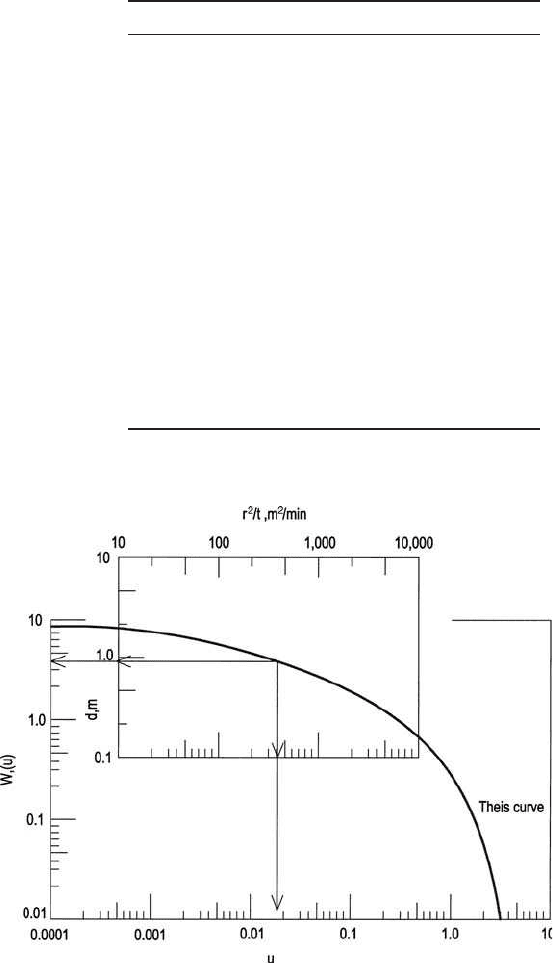
Figure 3.5 Observed data and Theis type curve.

solution:

Step 1. Calculate r

/t and construct a table with t and d

Step 2. Plot the observed data d versus r

/t on log-log (transparency) paper

in Fig. 3.5

Step 3. Plot a Theis type curve W(u) versus u on log-log paper (Fig. 3.5)

using the data listed in Appendix B (Illinois EPA, 1988)

Step 4. Select a match point on the superimposed plot of the observed data

on the type curve

Step 5. From the plots, the coordinates of the match points on the two curves

are

Observed data: r

/t ⫽ 320 m

/min

d ⫽ 0.90 m

Type curve: W(u) ⫽ 3.5

u ⫽ 0.018

Step 6. Substitute the above values to estimate T and S

Using Eq. (3.31)

Using Eq. (3.34)

5.2 Cooper–Jacob method

Cooper and Jacob (1946) modified the nonequilibrium equation. It is

noted that the parameter u in Eq. (3.32) becomes very small for large

5 2.30 3 10

S 5

4Tu

4 3 0.017 m

/s 3 0.018

320 m

/min 3 s1 min/60 sd

4Tu

5 0.017 m

T 5

QWsud

4pd

0.055 m

/s 3 3.5

4p 3 0.90 m

d 5

4pT

Wsud

Groundwater 201

values of t and small values of r. The infinite series for small u, W(u),

can be approximated by

(3.35)

Then

(3.36)

Further rearrangement and conversion to decimal logarithms yields

(3.37)

Therefore, the drawdown is to be a linear function of log t. A plot of d

versus the logarithm of t forms a straight line with the slope Q/4pT and

an intercept at d ⫽ 0, when t ⫽ t

, yielding

(3.38)

Since log(1) ⫽ 0

(3.39)

If the slope is measured over one log cycle of time, the slope will equal

the change in drawdown ⌬d, and Eq. (3.37) becomes

then

(3.40)

The Cooper and Jacob modified method solves for S and T when

values of u are less than 0.01. The method is not applicable to periods

immediately after pumping starts. Generally, 12 h or more of pumping

are required.

T 5

2.303Q

4p⌬d

⌬d 5

2.303Q

4pT

S 5

2.25Tt

1 5

2.25Tt

0 5

2.3Q

4pT

log

2.25Tt

d 5

2.303Q

4pT

log

2.25Tt

d 5

4pT

W sud 5

4pT

a20.5772 2 ln

4Tt

Wsud 520.5772 2 ln u 520.5772 2 ln

4Tt

202 Chapter 3

Example: Using the given data in the above example (by the Theis method)

with the Cooper and Jacob method, estimate the transmissivity and stora-

tivity of a confined aquifer.

solution:

Step 1. Determine t

and ⌬d

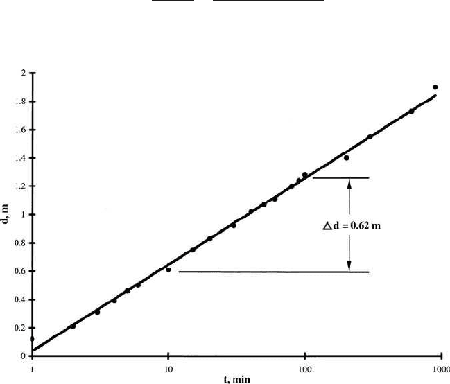
Values of drawdown (d) and time (t) are plotted on semilog paper with the t

in the logarithmic scale as shown in Fig. 3.6. A best-fit straight line is drawn

through the observed data. The intercept of the t-axis is 0.98 min. The slope

of the line ⌬d is measured over 1 log cycle of t from the figure. We obtain:

⫽ 0.98 min

⫽ 58.8 s

and for a cycle (t ⫽ 10 to 100 min)

⌬d ⫽ 0.62 m

Step 2. Compute T and S

Using Eq. (3.40)

5 0.016 m

T 5

2.303Q

4p⌬d

2.303 3 0.055 m

4 3 3.14 3 0.62 m

Groundwater 203

Figure 3.6 Relationship of drawdown and the time of pumping.

Using Eq. (3.39)

5.3 Distance-drawdown method

The distance-drawdown method is a modification of the Cooper and

Jacob method and is applied to obtain quick information about the

aquifer characteristics while the pumping test is in progress. The method

needs simultaneous observations of drawdown in three or more obser-

vation wells. The aquifer properties can be determined from pumping

tests by the following equations (Watson and Burnett, 1993):

(3.41)

(3.42)

and

(3.43)

(3.44)

where T ⫽ transmissivity, m

/d or gpd/ft

Q ⫽ normal discharge rate, m

/d or gpm

⌬(h

– h) ⫽ drawdown per log cycle of distance, m or ft

S ⫽ storativity, unitless

t ⫽ time since pumping when the simultaneous readings

are taken in all observation wells, days or min

⫽ intercept of the straight-line plot with the zero-

drawdown axis, m or ft

The distance-drawdown method involves the following procedures:

1. Plot the distance and drawdown data on semilog paper; drawdown

on the arithmetic scale and the distance on the logarithmic scale.

2. Read the drawdown per log cycle in the same manner for the Cooper

and Jacob method: this gives the value of ⌬(h

– h).

S 5

4790r

for English units

S 5

2.25Tt

for SI units

T 5

528Q

⌬sh

2 hd

for English units

T 5

0.366Q

⌬sh

2 hd

for SI units

5 2.61 3 10

S 5

2.25Tt

2.25 3 0.016 m

/s 3 58.8 s

s90 md

204 Chapter 3