Lee K.K. Lectures on Dynamical Systems, Structural Stability and Their Applications
Подождите немного. Документ загружается.

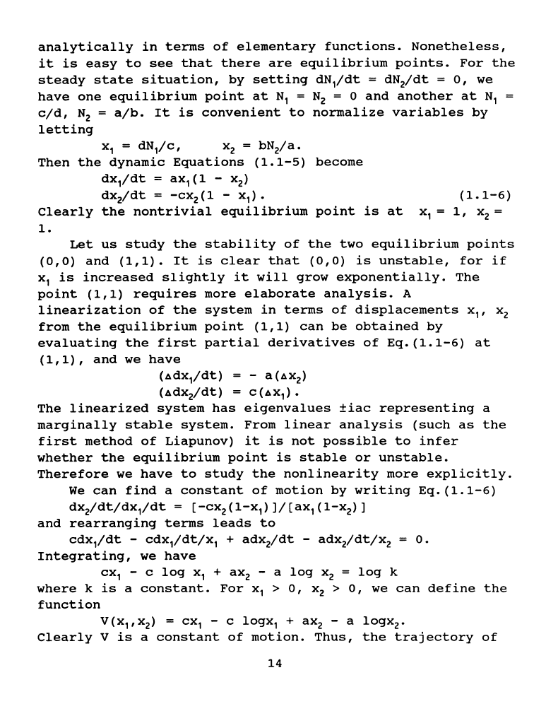
analytically
in
terms
of
elementary
functions.
Nonetheless,
it
is
easy
to
see
that
there
are
equilibrium
points.
For
the
steady
state
situation,
by
setting
dN
1
/dt
=
dN
2
/dt
= o,
we
have
one
equilibrium
point
at
N
1
= N
2
= 0
and
another
at
N
1
cjd,
N
2
=
ajb.
It
is
convenient
to
normalize
variables
by
letting
x
1
=
dN
1
jc,
x
2
=
bN
2
/a.
Then
the
dynamic
Equations
(1.1-5)
become
dx
1
jdt
=
ax
1
(1
- x
2
)
dx
2
jdt
=
-cx
2
(1
- x
1
).
(1.1-6)
Clearly
the
nontrivial
equilibrium
point
is
at
x
1
=
1,
x
2
=
1.
Let
us
study
the
stability
of
the
two
equilibrium
points
(0,0)
and
(1,1).
It
is
clear
that
(O,O)
is
unstable,
for
if
x
1
is
increased
slightly
it
will
grow
exponentially.
The
point
(1,1)
requires
more
elaborate
analysis.
A
linearization
of
the
system
in
terms
of
displacements
x
1
,
x
2
from
the
equilibrium
point
(1,1)
can
be
obtained
by
evaluating
the
first
partial
derivatives
of
Eq.(1.1-6)
at
(1,1),
and
we
have
(AdX
1
jdt)
= - a
(AX
2
)
(AdX
2
jdt)
=
C(AX
1
).
The
linearized
system
has
eigenvalues
±iac
representing
a
marginally
stable
system.
From
linear
analysis
(such
as
the
first
method
of
Liapunov)
it
is
not
possible
to
infer
whether
the
equilibrium
point
is
stable
or
unstable.
Therefore
we
have
to
study
the
nonlinearity
more
explicitly.
we
can
find
a
constant
of
motion
by
writing
Eq.(1.1-6)
dx
2
jdtjdx
1
/dt
=
[-cx
2
(1-x
1
)
]/
[ax
1
(1-x
2
)]
and
rearranging
terms
leads
to
cdx
1
jdt
-
cdx
1
jdtjx
1
+
adx
2
jdt
-
adx
2
jdtjx
2
0.
Integrating,
we
have
cx
1
-
c
log
x
1
+
ax
2
-
a
log
x
2
=
log
k
where
k
is
a
constant.
For
x
1
>
O,
x
2
> o, we
can
define
the
function
V(x
1
,x
2
)
=
cx
1
-
c
logx
1
+
ax
2
-
a
logx
2
•
Clearly
V
is
a
constant
of
motion.
Thus,
the
trajectory
of
14
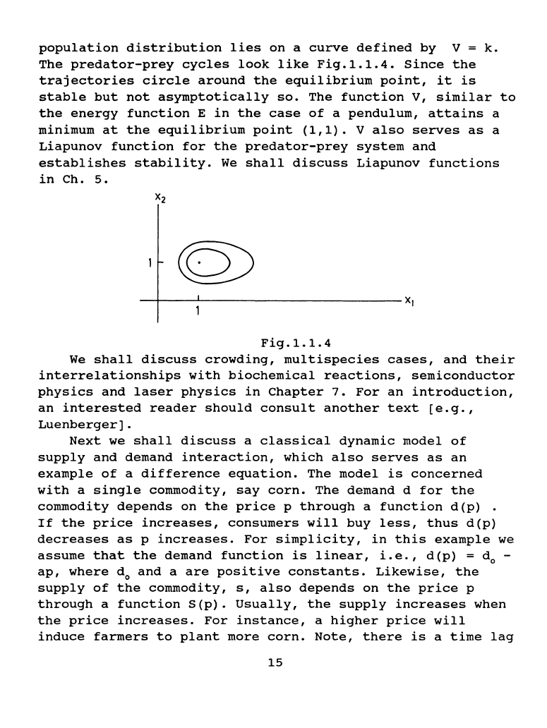
population
distribution
lies
on
a
curve
defined
by
V =
k.
The
predator-prey
cycles
look
like
Fig.1.1.4.
Since
the
trajectories
circle
around
the
equilibrium
point,
it
is
stable
but
not
asymptotically
so.
The
function
V,
similar
to
the
energy
function
E
in
the
case
of
a
pendulum,
attains
a
minimum
at
the
equilibrium
point
(1,1).
V
also
serves
as
a
Liapunov
function
for
the
predator-prey
system
and
establishes
stability.
We
shall
discuss
Liapunov
functions
in
Ch.
5.
--f-----L----------------------------XI
Fig
.1.
1.
4
We
shall
discuss
crowding,
multispecies
cases,
and
their
interrelationships
with
biochemical
reactions,
semiconductor
physics
and
laser
physics
in
Chapter
7.
For
an
introduction,
an
interested
reader
should
consult
another
text
[e.g.,
Luenberger]
.
Next
we
shall
discuss
a
classical
dynamic
model
of
supply
and
demand
interaction,
which
also
serves
as
an
example
of
a
difference
equation.
The
model
is
concerned
with
a
single
commodity,
say
corn.
The
demand
d
for
the
commodity
depends
on
the
price
p
through
a
function
d(p)
If
the
price
increases,
consumers
will
buy
less,
thus
d(p)
decreases
as
p
increases.
For
simplicity,
in
this
example
we
assume
that
the
demand
function
is
linear,
i.e.,
d(p)
= d
0
-
ap,
where
d
0
and
a
are
positive
constants.
Likewise,
the
supply
of
the
commodity,
s,
also
depends
on
the
price
p
through
a
function
S(p).
Usually,
the
supply
increases
when
the
price
increases.
For
instance,
a
higher
price
will
induce
farmers
to
plant
more
corn.
Note,
there
is
a
time
lag
15
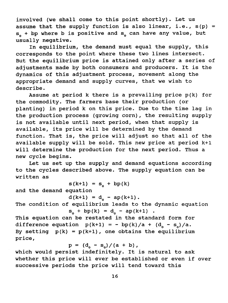
involved
(we
shall
come
to
this
point
shortly).
Let
us
assume
that
the
supply
function
is
also
linear,
i.e.,
s(p)
s
0
+
bp
where
b
is
positive
and
s
0
can
have
any
value,
but
usually
negative.
In
equilibrium,
the
demand
must
equal
the
supply,
this
corresponds
to
the
point
where
these
two
lines
intersect.
But
the
equilibrium
price
is
attained
only
after
a
series
of
adjustments
made
by
both
consumers
and
producers.
It
is
the
dynamics
of
this
adjustment
process,
movement
along
the
appropriate
demand
and
supply
curves,
that
we
wish
to
describe.
Assume
at
period
k
there
is
a
prevailing
price
p(k)
for
the
commodity.
The
farmers
base
their
production
(or
planting)
in
period
k
on
this
price.
Due
to
the
time
lag
in
the
production
process
(growing
corn),
the
resulting
supply
is
not
available
until
next
period,
when
that
supply
is
available,
its
price
will
be
determined
by
the
demand
function.
That
is,
the
price
will
adjust
so
that
all
of
the
available
supply
will
be
sold.
This
new
price
at
period
k+l
will
determine
the
production
for
the
next
period.
Thus
a
new
cycle
begins.
Let
us
set
up
the
supply
and
demand
equations
according
to
the
cycles
described
above.
The
supply
equation
can
be
written
as
s(k+l)
= s
0
+
bp(k)
and
the
demand
equation
d(k+l)
= d
0
-
ap(k+l).
The
condition
of
equilibrium
leads
to
the
dynamic
equation
S
0
+
bp(k)
= d
0
-
ap(k+l)
.
This
equation
can
be
restated
in
the
standard
form
for
difference
equation
p(k+l)
= -
bp(k)/a
+
(d
0
- S
0
)/a.
By
setting
p(k)
=
p(k+l),
one
obtains
the
equilibrium
price,
p =
(d
0
-
s
0
)/(a
+b),
which
would
persist
indefinitely.
It
is
natural
to
ask
whether
this
price
will
ever
be
established
or
even
if
over
successive
periods
the
price
will
tend
toward
this
16
equilibrium
price
and
not
diverge
away
from
it.
From
the
general
solution
of
the
first-
order
equation
we
have
p(k)
=
(-b/a)kp(O)
+
[1-(-b/a)k]
(d
0
-
S
0
)/(a
+
b).
If
b <
a,
it
follows
that
as
k
~
~
the
solution
will
tend
toward
the
equilibrium
value
since
all
(-
b/a)k
terms
go
to
zero
and
the
equilibrium
value
is
independent
of
the
initial
price.
Clearly,
b < a
is
both
necessary
and
sufficient
for
this
convergence
property
to
hold.
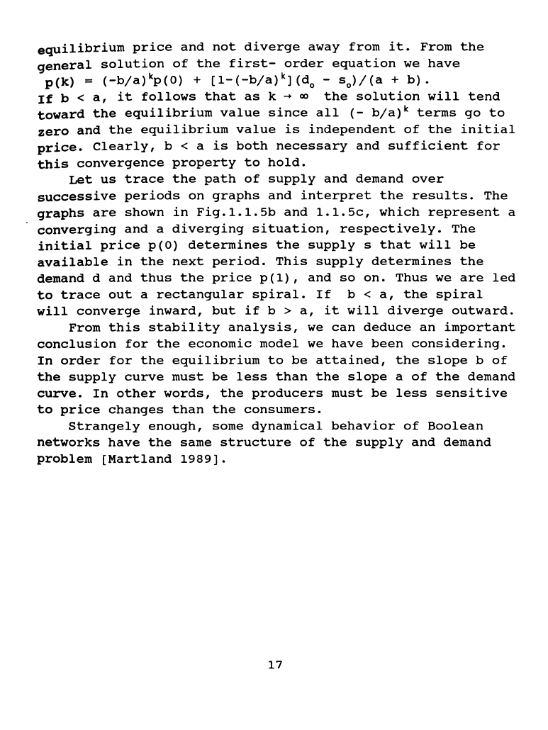
Let
us
trace
the
path
of
supply
and
demand
over
successive
periods
on
graphs
and
interpret
the
results.
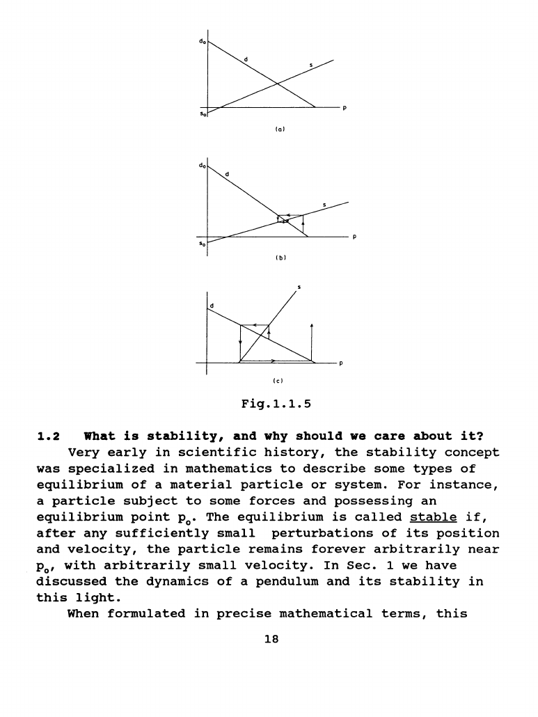
The
graphs
are
shown
in
Fig.1.1.5b
and
1.1.5c,
which
represent
a
converging
and
a
diverging
situation,
respectively.
The
initial
price
p(O)
determines
the
supply
s
that
will
be
available
in
the
next
period.
This
supply
determines
the
demand d
and
thus
the
price
p(1),
and
so
on.
Thus
we
are
led
to
trace
out
a
rectangular
spiral.
If
b <
a,
the
spiral
will
converge
inward,
but
if
b >
a,
it
will
diverge
outward.
From
this
stability
analysis,
we
can
deduce
an
important
conclusion
for
the
economic
model
we
have
been
considering.
In
order
for
the
equilibrium
to
be
attained,
the
slope
b
of
the
supply
curve
must
be
less
than
the
slope
a
of
the
demand
curve.
In
other
words,
the
producers
must
be
less
sensitive
to
price
changes
than
the
consumers.
Strangely
enough,
some
dynamical
behavior
of
Boolean
networks
have
the
same
structure
of
the
supply
and
demand
problem
[Hartland
1989].
17
lol
lcl
Fig.1.1.5
1.2
What
is
stability,
and
why
should
we
care
about
it?
Very
early
in
scientific
history,
the
stability
concept
was
specialized
in
mathematics
to
describe
some
types
of
equilibrium
of
a
material
particle
or
system.
For
instance,
a
particle
subject
to
some
forces
and
possessing
an
equilibrium
point
p
0
•
The
equilibrium
is
called
stable
if,
after
any
sufficiently
small
perturbations
of
its
position
and
velocity,
the
particle
remains
forever
arbitrarily
near
p
0
,
with
arbitrarily
small
velocity.
In
Sec.
1
we
have
discussed
the
dynamics
of
a
pendulum
and
its
stability
in
this
light.
When
formulated
in
precise
mathematical
terms,
this
18
mechanical
definition
of
stability
was
found
useful
in
many
situations,
but
inadequate
in
many
others.
This
is
why,
over
the
years,
a
host
of
other
concepts
have
been
introduced,
each
of
them
related
to
the
first
mechanical
definition
and
to
the
common
sense
of
stability.
In
contrast
to
the
mechanical
definition
of
stability,
the
concept
known
as
Liapunov•s
stability
has
the
following
characteristics:
(i)
it
pertains
not
to
a
material
particle
or
the
particular
equation,
but
to
a
general
differential
equation;
(ii)
it
applies
to
a
solution,
thus
not
only
to
an
equilibrium
or
critical
point.
More
precisely,
let
dx/dt
=
f(t,x)
(1.2-1)
where
x
and
f
are
real
n-vectors,
t £ R
is
the
time,
f
is
defined
on
R x R".
We
also
assume
f
is
smooth
enough
to
ensure
the
exsistence,
uniqueness
and
continuous
dependence
of
the
solutions
of
the
initial
value
problem
associated
with
Eq.
(1.2-1)
over
R x R".
Let
11·11
denote
any
norm
on
R".
A
solution
x(t)
of
Eq.(1.2-1)
is
stable
at
t
0
,
or
at
t = t
0
in
the
sense
of
Liapunov
if,
for
every
£ > o,
there
is
a 6 >
0
such
that
if
x•
(t)
is
any
other
solution
with
llx•
(t
0
)
-
x(t
0
)ll <
6,
then
llx•(t)-
x(t)ll
<£for
all
t > t
0
•
Otherwise,
x(t)
is
unstable
at
t
0
•
Thus,
stability
at
t
0
is
nothing
but
continuous
dependence
of
the
solutions
on
X
1
0
=
X
1
(t
0
),
uniform
with
respect
tot£
[t,~
).
Notice
that
in
the
case
of
the
pendulum,
the
equilibrium
point
(0,0)
in
the
phase
space
is
such
that
no
neighboring
solution
approaches
it
when t
~
~
,
except
if
some
friction
were
present.
In
many
practical
situations,
it
is
useful
to
require,
in
addition
to
Liapunov
stability
of
a
solution
x(t),
that
all
neighboring
solutions
x•(t)
tend
to
x(t)
when
t
~
~
•
This
leads
to
the
notion
of
asymptotic
stability.
Many
other
examples
can
illustrate
the
necessity
of
creating
new
specific
concepts.
Indeed,
the
stability
of
relative
equilibria
in
celestial
mechanics
is
subtle,
to
say
the
least,
depending
on
deep
properties
of
Hamiltonian
systems
(as
has
been
shown
by
Kolmogorov
[1954],
Moser
[1962],
Arnold
[1963a,b)
and
Russman
[1970]),
it
is
known
as
19
the
Kolmogorov-Arnold-Moser
(KAM)
theorem.
We
shall
briefly
discuss
this
theorem
in
Section
2.8.
For
further
reading
of
KAM
theorem,
consult,
for
instance,
Abraham
and
Marsden
[1978],
or
Arnold
[1978].
From common
sense,
the
solar
system
is
considered
stable
because
it
is
durable,
i.e.,
none
of
its
planets
escapes
to
infinity,
nor
do
any
two
such
planets
collide.
But
the
velocities
are
unbounded
iff
two
bodies
approach
each
other.
Therefore,
the
Lagrange
stability
simply
means
that
the
coordinates
and
velocities
of
the
bodies
are
bounded.
Thus
boundedness
of
the
solution
appears
as
a
legitimate
and
natural
type
of
stability.
For
many
other
definitions
of
stability
and
attractivity,
please
see
Rouche,
Habets
&
Laloy
[1977].
The
most
comprehensive
of
many
different
notions
of
stability
is
the
problem
of
structural
stability.
This
problem
asks:
If
a
dynamical
system
X
has
a known
phase
portrait
P,
and
X
is
then
perturbed
to
a
slightly
different
system
X'
(such
as,
changing
the
coefficients
in
the
differential
equations
slightly),
then
is
the
new
phase
portrait
P'
close
to
P
in
some
topological
sense?
This
problem
has
obvious
importance,
because
in
practice
the
qualitative
information
obtained
for
P
is
not
applied
to
X
but
to
some
nearby
system
X'.
This
is
because
the
coefficients
of
the
equation
are
determined
experimentally
,
thus
approximately.
An
important
role
physics
plays
in
various
disciplines
of
science
is
that
most
systems
and
structures
in
nature
enjoy
an
inherent
"physical
stability",
i.e.,
they
preserve
their
quality
under
slight
perturbations-
i.e.,
they
are
structurally
stable.
Otherwise
we
could
hardly
think
about
or
describe
them,
and
reproducibility
and
confirmation
of
experiments
would
not
be
possible.
Thus
we
have
to
accept
structural
stability
as
a
fundamental
principle,
which
not
only
complements
the
known
physical
laws,
but
also
serves
as
a
foundation
upon
which
these
physical
laws
are
built.
Thus
universal
phenomena
have
a common
topological
origin,
and
they
are
describable
and
classifiable
by
unfoldings
of
20
sinqularities,
which
orqanize
the
bifurcation
processes
exhibited
by
dynamical
systems.
Here
bifurcation
refers
to
the
chanqes
in
the
qualitative
structure
of
solutions
of
differential
equations
describinq
the
qoverninq
dynamical
systems.
A
phenomenon
is
said
to
be
structurally
stable
if
it
persists
under
all
allowed
perturbations
in
the
system.
Another
important
approach
or
"utility"
of
structural
stability
analysis
is
the
followinq.
Since
most
of
the
nonlinear
equations
of
nature
are
not
amenable
to
a
quantitative
analysis,
only
a
few
are
known.
Consequently
it
is
often
unclear
which
particular
quantitative
effects
one
ouqht
to
study.
Nonetheless,
since
the
nonlinear
equations
are
derived
from
qeometrical
or
topoloqical
invariance
principles,
they
must
process
structurally
stable
solutions.
In
determininq
these
stable
solutions
qualitatively,
it
will
provide
us
with
conceptual
quidance
to
sinqle
out
the
most
siqnificant
phenomena
in
complex
systems
to
answer
the
questions
of
structure
formation
and
recoqnition.
Traditionally,
the
usefulness
of
a
theory
is
judqed
by
the
criterion
of
adequacy,
i.e.,
the
verifiability
of
the
predictions,
or
the
quality
of
the
aqreement
between
the
interpreted
conclusions
of
the
model
and
the
data
of
the
experiments.
Duhem
adds
the
criterion
of
stability.
This
criterion
refers
to
the
stability
or
continuity
of
the
predictions,
or
their
adequacy
when
the
model
is
sliqhtly
perturbed.
And
the
qeneral
applicability
of
this
type
of
criterion
has
been
suqqested
by
Them
[1973].
This
stability
concerns
variation
of
the
model
only,
the
interpretation
and
experimental
domain
beinq
fixed.
Therefore
it
mainly
concerns
the
model,
and
is
primarily
a
mathematical
or
loqical
question.
It
is
safe
to
say
that
a
clear
enunciation
of
this
criterion
in
the
correct
qenerality
has
not
yet
been
made,
although
some
proqress
has
been
made
recently.
A
tacit
assumption
(or
criterion)
which
has
been
implicitly
adapted
by
physicists
may
be
called
the
doctrine
of
stability.
For
instance,
in
a
model
of
a
system
with
differential
equations
where
the
model
depends
on
some
21
parameters
or
some
coefficients
of
the
differential
equations,
each
set
of
values
corresponds
to
a
different
model.
As
these
parameters
can
be
determined
approximately,
the
theory
is
useful
only
if
the
equations
are
structurally
stable,
which
cannot
be
proved
at
present
in
many
important
cases.
Thus
physicists
must
rely
on
faith
at
this
moment.
Thom
[1973]
offered
an
alternative
to
the
doctrine
of
stability.
He
suggested
that
stability,
when
precisely
formulated
in
a
specific
theory,
could
be
added
to
the
model
as
an
additional
hypothesis.
This
formalization
reduces
the
criterion
of
stability
to
an
aspect
of
the
criterion
of
adequacy,
and
may
admit
additional
theorems
or
predictions
in
the
model.
Although
no
implications
of
this
axiom
is
known
for
celestial
mechanics
as
yet,
Thom
has
described
some
conclusions
in
his
model
for
biological
systems.
A
careful
statement
of
this
notion
of
stability
in
the
general
context
of
physical
sciences
and
epistemology,
just
to
name
a
few
disciplines,
could
be
quite
useful
in
technical
applications
of
mechanics
as
well
as
in
the
formation
of
new
qualitative
theories
in
physical,
biological,
and
social
sciences.
In
all
fields
of
physics,
waves
are
used
to
investigate
(probe)
some unknown
structures.
such
a
structure
or
object
impresses
geometrical
singularity
upon
smooth
incident
wavefields.
The
question
is
then,
what
information
about
the
structure
under
study
can
be
inferred
from
these
geometrical
singularities;
this
is
the
so-called
inverse
scattering
problem.
In
order
that
the
reconstruction
of
structures
from
the
backscattered
or
transmitted
curves
will
be
physically
repeatable,
the
scattering
process
has
to
be
structurally
stable,
that
is,
qualitatively
insensitive,
to
slight
perturbations
of
the
wavefields.
Imposing
this
structural
stability
principle
on
the
inverse
scattering
process
allows
us
to
classify
the
geometrical
singularities,
impresses
on
the
sensing
wavefields
by
the
unknown
structure,
into
a
few
universal
topological
normal
forms
described
by
catastrophe
22
polynomials.
Moreover,
the
topological
singularities
provide
an
explanation
for
the
similarity
and
universality
of
the
patterns
encountered
in
geophysics
and
seismology
(Dangelmay
and
Guttinger
1982,
Hilterman
1975],
ocean
acoustics
(Keller
and
Papadakis
1977],
optics
(Baltes
1980,
Berry
1977,
Nye
1978,
Berry
1980],
and
various
topography,
etc.
On
a
more
fundamental
level,
nonlinear
dynamical
systems
and
their
stability
analyses
have
clearly
demonstrated
the
unexpected
fact
that
systems
governed
by
the
Newtonian
dynamics
do
not
necessarily
exhibit
the
usual
"predictability"
property
as
expected.
Indeed,
a
wide
classes
of
even
very
simple
systems,
which
satisfy
those
Newtonian
equations,
predictability
is
impossible
beyond
a
certain
definite
time
horizon.
This
failure
of
predictability
in
Newtonian
dynamics
has
been
very
well
elucidated
in
a
review
paper
by
Lighthill
(1986].
Moreover,
recently,
there
have
been
several
papers
attempting
to
relate
such
unpredictability
to
statistical
mechanics.
Nonetheless,
a much
more
fundamental
framework
together
with
appropriate
mathematical
structure
have
to
be
established
before
any
such
correlation
can
be
made.
In
the
next
chapter,
we
shall
assemble
some
of
the
definitions
and
theorems,
without
proof,
about
basic
properties
of
algebra,
topology,
and
differential
geometry,
which
are
essential
to
our
discussion
of
the
geometric
theory
of
nonlinear
dynamical
systems.
23
