Lalanne C. Mechanical Vibrations and Shocks: Mechanical Shock Volume II
Подождите немного. Документ загружается.

4
Mechanical shock
1.1.11.
Versed-sine
(or
haversine) shock
Simple
shock
for
which
the
acceleration-time curve
has the
form
of one
period
of
the
curve representative
of the
function
[1 -
cos(
)],
with this period starting
from
zero value
of
this
function.
It is
thus
a
signal ranging between
two
minima.
1.1.12.
Decaying
sinusoidal
pulse
A
pulse comprised
of a few
periods
of a
damped sinusoid, characterized
by the
amplitude
of the first
peak,
the frequency and
damping:
This
form
is
interesting,
for it
represents
the
impulse response
of a
one-degree-
of-freedom
system
to a
shock.
It is
also used
to
constitute
a
signal
of a
specified
shock
response
spectrum (shaker control
from a
shock response spectrum).
1.2.
Analysis
in the
time domain
A
shock
can be
described
in the
time domain
by the
following
parameters:
-
the
amplitude x(t);
-
duration
t;
-
the
form.
The
physical parameter expressed
in
terms
of
time
is, in a
general way,
an
acceleration x(t),
but can be
also
a
velocity v(t),
a
displacement x(t)
or a
force
F(t).
In
the
first
case,
which
we
will particularly consider
in
this volume,
the
velocity
change
corresponding
to the
shock movement
is
equal
to
1.3.
Fourier transform
1.3.1.
Definition
The
Fourier integral
(or
Fourier transform)
of a
function
x(t)
of the
real variable
t
absolutely integrable
is
defined
by
Shock analysis
5
The
function X(Q)
is in
general complex
and can be
written,
by
separating
the
real
and
imaginary parts
${(£1)
and
3(Q):
or
with
and
Thus
is
the
Fourier spectrum
of
I
the
energy
spectrum
and
is
the
phase.
The
calculation
of the
Fourier transform
is a
one-to-one operation.
By
means
of
the
inversion
formula
or
Fourier
reciprocity
formula.,
it is
shown that
it is
possible
to
express
in a
univocal
way
x(t) according
to its
Fourier transform X(Q)
by the
relation
(if the
transform
of
Fourier X(Q)
is
itself
an
absolutely integrable
function
over
all
the
domain).
NOTES.
I.
For
dt
6
Mechanical shock
The
ordinate
at f = 0
of
the
Fourier
transform
(amplitude)
of
a
shock
defined
by
an
acceleration
is
equal
to the
velocity change
AV
associated with
the
shock
(area
under
the
curve x(t)).
2.
The
following
definitions
are
also
sometimes
found
[LAL
75]:
In
this last case,
the two
expressions
are
formally
symmetrical.
The
sign
of
the
exponent
of
exponential
is
sometimes also selected
to be
positive
in the
expression
for
X(Q)
and
negative
in
that
for
x(t).
1.3.2.
Reduced Fourier
transform
The
amplitude
and the
phase
of the
Fourier transform
of a
shock
of
given shape
can
be
plotted
on
axes where
the
product
f T (T =
shock duration)
is
plotted
on the
abscissa
and on the
ordinate,
for the
amplitude,
the
quantity
A(f
)/x
m
r .
In
the
following paragraph,
we
draw
the
Fourier spectrum
by
considering simple
shocks
of
unit duration (equivalent
to the
product
ft) and of the
amplitude unit.
It
is
easy, with this representation,
to
recalibrate
the
scales
to
determine
the
Fourier
spectrum
of a
shock
of the
same form,
but of
arbitrary duration
and
amplitude.
Shock analysis
7
1.3.3.
Fourier
transforms
of
simple
shocks
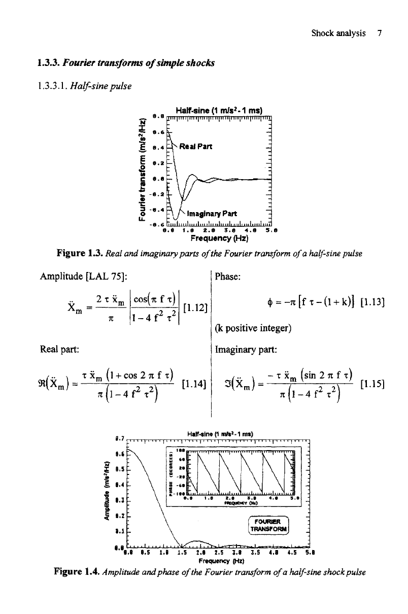
1.3.3.1.
Half-sine
pulse
Figure
1.3.
Real
and
imaginary
parts
of
the
Fourier
transform
of
a
half-sine
pulse
Amplitude
[LAL 75]:
Phase:
(k
positive integer)
Imaginary
part:
Real
part:
Figure
1.4.
Amplitude
and
phase
of
the
Fourier
transform
of
a
half-sine
shock pulse
8
Mechanical shock
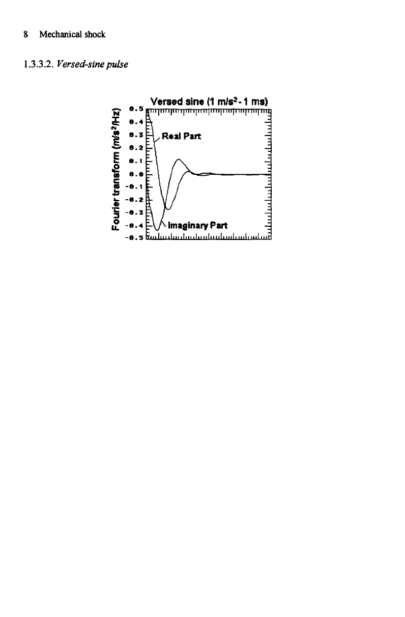
1.3.3.2.
Versed-sine
pulse
Figure
1.5. Real
and
imaginary parts
of
the
Fourier
transform
of
a
versed-sine shock pulse
Amplitude:
Phase:
Imaginary part:
Real part:
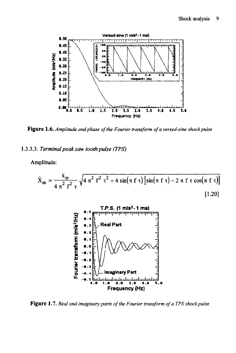
Shock
analysis
9
Figure 1.6.
Amplitude
and
phase
of
the
Fourier
transform
of
a
versed-sine shockpulse
1.3.3.3.
Terminal
peak
saw
tooth pulse
(TPS)
Amplitude:
Figure
1.7.
Real
and
imaginary
parts
of
the
Fourier
transform
of
a
TPS
shockpulse
10
Mechanical
shock
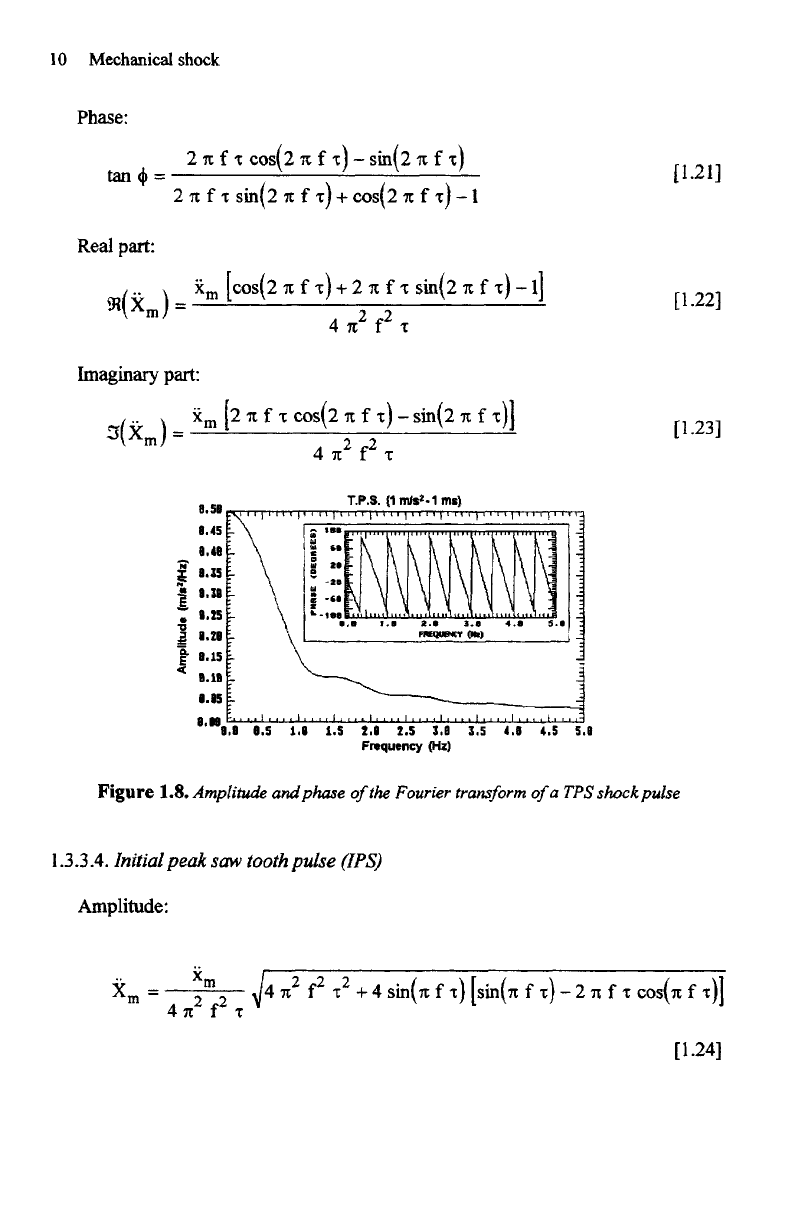
Phase:
Real
part:
Imaginary
part:
Figure
1.8.
Amplitude
and
phase
of
the
Fourier
transform
of
a
TPS
shock
pulse
1.3.3.4.
Initial
peak
saw
tooth pulse
(IPS)
Amplitude:
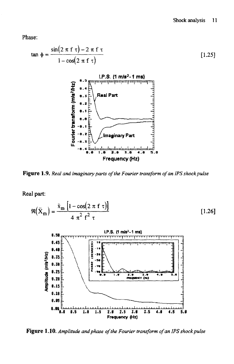
Phase:
Shock analysis
11
Figure
1.9. Real
and
imaginary
parts
of
the
Fourier
transform
of
an IPS
shock pulse
Real
part:
Figure
1.10. Amplitude
and
phase
of
the
Fourier
transform
of
an IPS
shock pulse
12
Mechanical shock
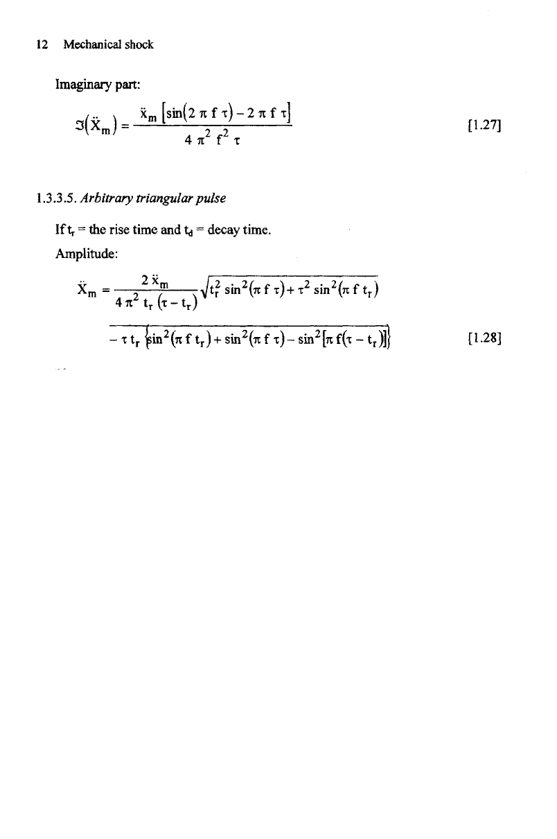
Imaginary part:
1.3.3.5.
Arbitrary
triangular
pulse
If
tr
= the
rise time
and t^ =
decay time.
Amplitude:
Phase:
Real part:
Shock
analysis
13
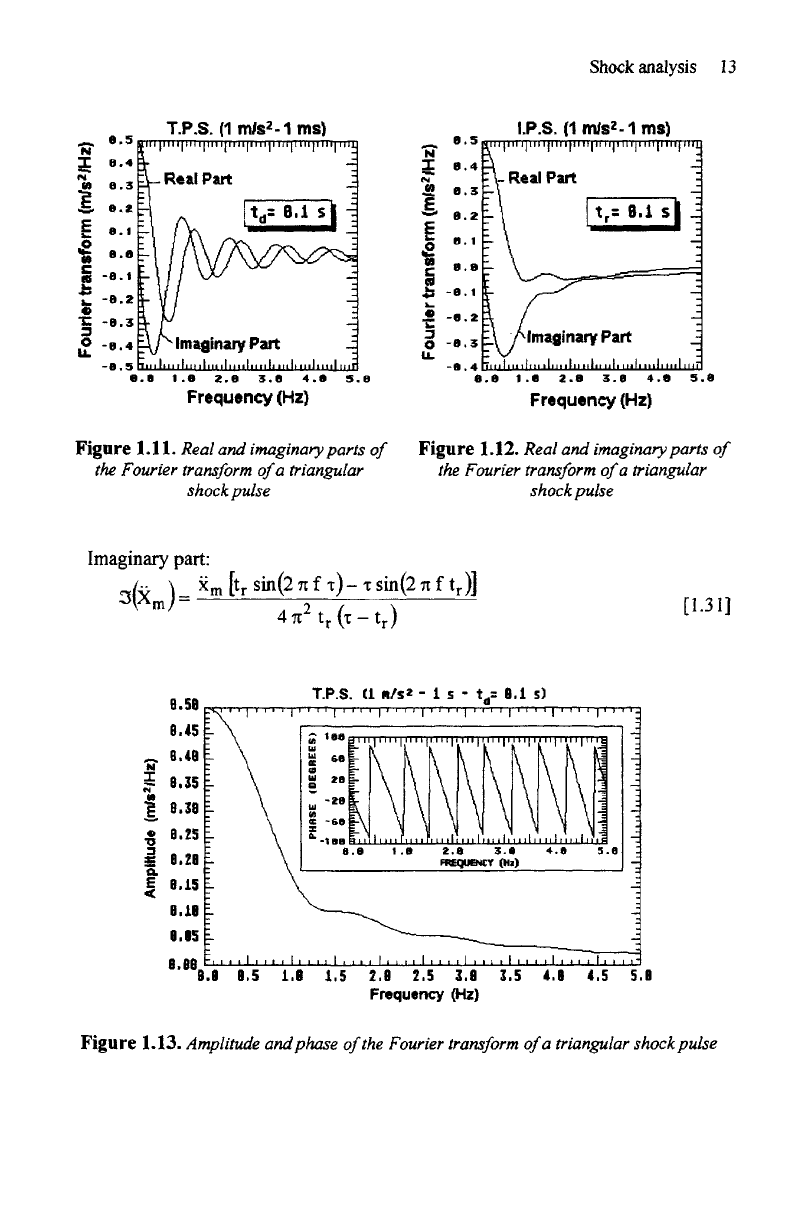
Figure
1.11. Real
and
imaginary
parts
of
the
Fourier
transform
of
a
triangular
shock
pulse
Figure
1.12. Real
and
imaginary
parts
of
the
Fourier
transform
of
a
triangular
shock pulse
Imaginary
part:
Figure
1.13. Amplitude
and
phase
of
the
Fourier
transform
of
a
triangular shock pulse