Labelle P. Supersymmetry DeMYSTiFied
Подождите немного. Документ загружается.


186
Supersymmetry Demystified
To lowest order (order g
0
), we get
|T
A(x)
|=0|A(x)|0=0 (9.31)
because A(x) is a sum of single creation and annihilation operators. The first
nonzero contribution is of order g and is given by
|T
A(x)
|
g
=
d
4
z0|T
iA(x)(L
I 2
(z) + L
I 3
(z))
|0
=−ig
d
4
z0|T
mA(x) A
3
(z)
I
+mA(x) A(z)B
2
(z)
II
+ A(x) A(z)
III
(9.32)
Note that the interaction L
I 4
does not contribute because it does not contain any A
field to pair up with A(x). We haven’t written the denominator of Eq. (9.30) (whose
purpose is to remove the disconnected diagrams) because it is equal to one at the
order we are working.
In the first term of Eq. (9.32), we have three ways to contract A(x) with one of
the A(z) and only one way to contract the two remaining A(z) which gives us a
factor of 3. The first term is therefore
I =−3igm
d
4
zD
A
(x − z)D
A
(z − z)
=−3igm
d
4
z
d
4
q
(2π)
4
d
4
k
(2π)
4
ie
−iq·(x−z)
q
2
− m
2
+i
ie
−ik·(z−z)
k
2
− m
2
+i
=−3igm
d
4
z
d
4
q
(2π)
4
d
4
k
(2π)
4
ie
−iq·(x−z)
q
2
− m
2
+i
i
k
2
− m
2
+i
(9.33)
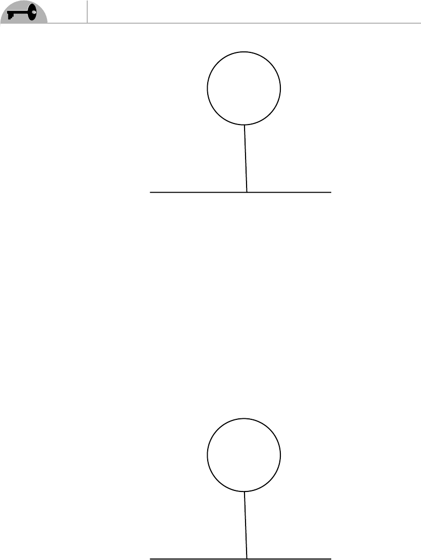
which is illustrated in Figure 9.2.
Carrying out the integral over z gives (2π
4
)δ
4
(q), which allows us to trivially
integrate over q, finally giving us
I =−
3ig
m
d
4
k
(2π)
4
1
k
2
− m
2
+i
=−3
g
m
I
d
(9.34)
with I
d
given in Eq.(9.15).
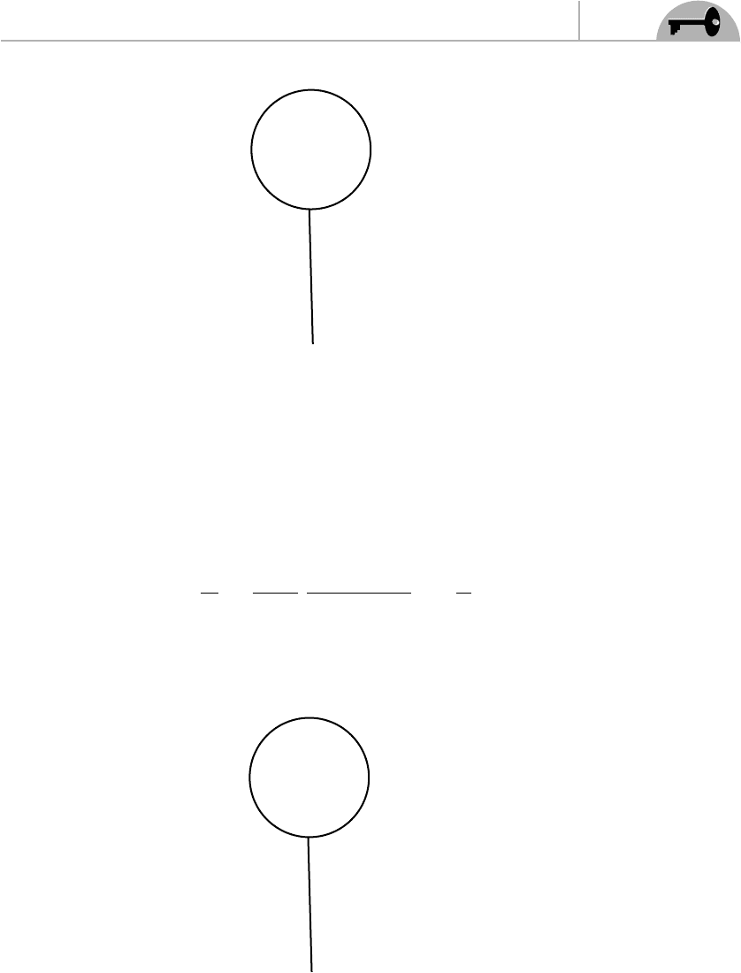
CHAPTER 9 Some Explicit Calculations
187
A
A
Figure 9.2 Diagram corresponding to Eq. (9.33).
Now look at the second term of Eq. (9.32). There is only one way to contract the
fields, so this contribution is simply
II =−igm
d
4
zD
a
(x − z)D
B
(z − z)
=−
ig
m
d
4
k
(2π)
4
1
k
2
− m
2
+i
=−
g
m
I
d
(9.35)
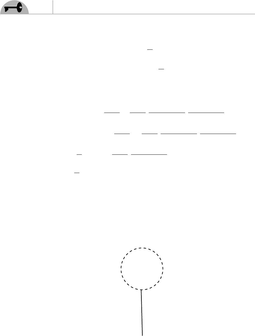
with the corresponding diagram illustrated in Figure 9.3.
A
B
Figure 9.3 Diagram corresponding to Eq. (9.35).
188
Supersymmetry Demystified
Finally, there is the third term of Eq. (9.32). It is equal to
III =−ig
d
4
zD
A
(x − z) 0|T
α
(z)
α
(z)
|0
= ig
d
4
zD
A
(x − z) 0|T
α
(z)
α
(z)
|0
= ig
d
4
zD
A
(x − z) Tr
S(z − z)
= ig
d
4
z
d
4
q
(2π)
4
d
4
k
(2π)
4
ie
−iq·(x−z)
q
2
− m
2
+i
iTr(/k +m)
k
2
− m
2
+i
= 4igm
d
4
z
d
4
q
(2π)
4
d
4
k
(2π)
4
ie
−iq·(x−z)
q
2
− m
2
+i
i
k
2
− m
2
+i
= 4i
g
m
d
4
z
d
4
k
(2π)
4
1
k
2
− m
2
+i
= 4
g
m
I
d
(9.36)
where we have used the usual trace identities for gamma matrices (which are
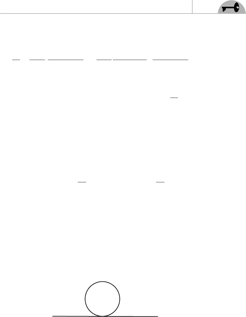
summarized in Appendix A). The corresponding Feynman diagram is shown in
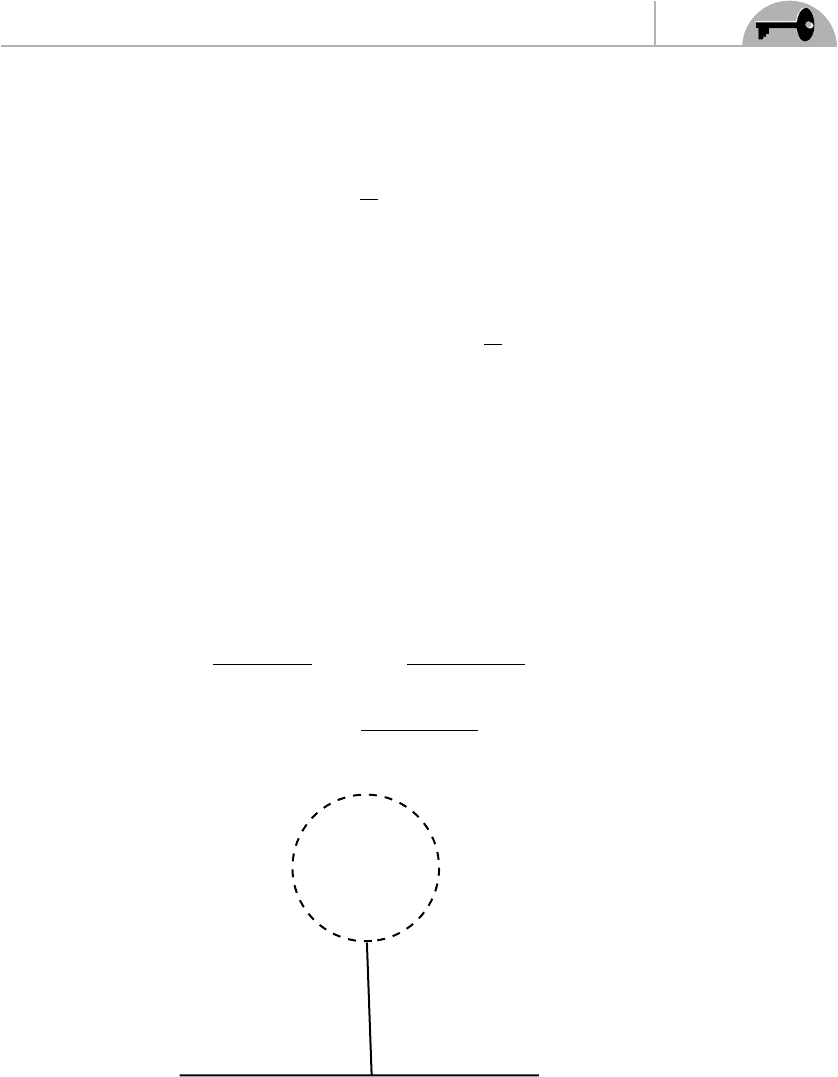
Figure 9.4.
The three terms in Eqs. (9.33), (9.35), and (9.36) are seen to cancel out exactly.
More specifically, the contribution from the fermion loop cancels out exactly the
contribution from the two scalar loops.
A
Ψ
Figure 9.4 Diagram corresponding to Eq. (9.36).

CHAPTER 9 Some Explicit Calculations
189
Note that this works only because the same coupling constant g appears in both
L
I 2
and L
I 3
and because the three particles have the same mass, which is also equal
to the parameter m appearing as a coupling constant in L
I 2
.
9.4 Propagator of the B Field to One Loop
We consider now
|T
B(x)B(y)
|=
0|T (B(x)B(y)e
i
d
4
zL
(z)
)|0
0|T (e
i
d
4
zL
(z)
)|0
(9.37)
Let us recall that the effect of the denominator is to remove the disconnected
diagrams from the perturbation expansion.
The lowest-order (order g
0
) contribution is simply the free-particle propagator
D
B
(x − y). There is no distinction between the free propagators of the A and B
fields because they have the same mass. However, we will still distinguish the two
by calling them D
A
and D
B
because it will be useful to distinguish the contribu-
tions of the two fields when we discuss SUSY spontaneous symmetry breaking in
Chapter 14.
The only way to have a nonzero result in the expansion of the exponential in the
numerator is to have an even number of A and B fields (if there is an odd number of
fields, there will always be a creation or annihilation operator that will be unpaired,
which, when sandwiched between the vacuum, will give zero). Because of this, we
can see that there is no order g contributions.
O(g
2
) contribution comes from the L
I 1
term in the first order of the expansion
of the exponential, i.e.,
d
4
z0|T
iB(x)B(y)L
I 1
(z)
|0 (9.38)
and six contributions from the second order of the expansion of the exponential,
i.e.,
d
4
z
d
4
w0|T
"
B(x)B(y)
−
1
2
L
I 2
(z)L
I 2
(w) −
1
2
L
I 3
(z)L
I 3
(w)
−
1
2
L
I 4
(z)L
I 4
(w) − L
I 2
(z)L
I 3
(w) − L
I 2
(z)L
I 4
(w) − L
I 3
(z)L
I 4
(w)
#
|0
(9.39)

190
Supersymmetry Demystified
A Few More Useful Integrals
The integral in Eq. (9.13) will be useful several times in this chapter. There are two
more integrals that will show up repeatedly. We will evaluate them here to alleviate
the presentation in the next few sections.
One of these integrals is
d
4
zd
4
wD(x − z)D(y − w)D(w − z)D(w − z)
=
d
4
zd
4
w
d
4
p
(2π)
4
ie
−ip·(x−z)
p
2
− m
2
+i
d
4
q
(2π)
4
ie
−iq·(y−w )
q
2
− m
2
+i
d
4
k
(2π)
4
ie
−ik·(w −z)
k
2
− m
2
+i
d
4
l
(2π)
4
ie
−il·(w−z)
l
2
− m
2
+i
Doing the z integration gives a factor (2π)
4
δ
4
( p + k +l). Integrating then over l,
over w, and finally, over q, we finally get
d
4
p
(2π)
4
e
−ip·(x−y)
i
p
2
− m
2
+i
i
p
2
− m
2
+i
×
d
4
k
(2π)
4
i
k
2
− m
2
+i
i
( p + k)
2
− m
2
+i
(9.40)
whose amputated Fourier transform is
d
4
zd
4
wD(x − z)D(y − w)D(w − z)D(w − z)
AM
FT
≡ I
log
(9.41)
where I
log
is the logarithmically divergent integral between brackets in Eq. (9.40).
The second integral we will often need is
d
4
zd
4
wD(x − z) D(y − z) D(z −w ) D(w − w)
=
d
4
zd
4
w
d
4
p
(2π)
4
ie
−ip·(x−z)
p
2
− m
2
+i
d
4
q
(2π)
4
ie
−iq·(y−z)
q
2
− m
2
+i
d
4
k
(2π)
4
ie
−ik·(z−w )
k
2
− m
2
+i
d
4
l
(2π)
4
ie
−il·(w−w)
l
2
− m
2
+i
(9.42)
CHAPTER 9 Some Explicit Calculations
191
Doing the z integration, we get a factor (2π)
4
δ
4
( p + q −k) that we may use to
integrate over k. Integrating then over w and finally over q,weget
−
i
m
2
d
4
p
(2π)
4
ie
−ip·(x−y)
p
2
− m
2
+i
d
4
l
(2π)
4
i
l
2
− m
2
+i
i
p
2
− m
2
+i
(9.43)
so the Fourier transform of Eq. (9.42) is (after amputating the external lines)
d
4
zd
4
wD(x − z)D(y − z)D(z −w )D(w − w)
AM
FT
=−
i
m
2
I
d
(9.44)
with I
d
defined in Eq. (9.13).
Now we are well equipped to calculate the one-loop corrections to the B propa-
gator.
Contribution from L
I1
Consider first the contribution from L
I 1
[see Eqs. (9.38) and (8.71)]. It is
d
4
z0|T
"
B(x)B(y)
−
ig
2
2
B(z)
4
−ig
2
A(z)
2
B(z)
2
−
ig
2
2
A(z)
4
#
|0
(9.45)
In the first term, there are four ways to contract B(x) with one of the B(z). Then
there are three ways to contract B(y) with one of the remaining B(z). The two B(z)
left over must be contracted together. We therefore get
−6ig
2
d
4
zD
B
(x − z)D
B
(y − z)D
B
(z − z)
AM
FT
=−6ig
2
I
d
(9.46)
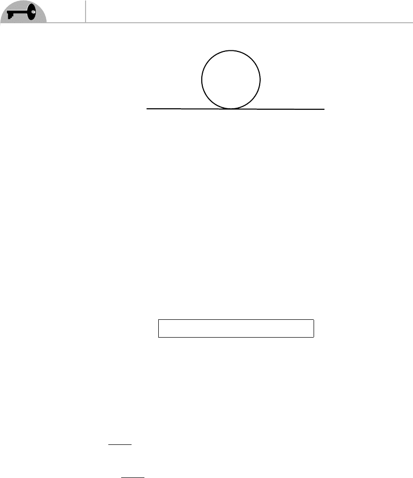
where we have used Eq. (9.12). This integral corresponds to Figure 9.5.
B
B
B
Figure 9.5 Diagram corresponding to Eq. (9.46).
192
Supersymmetry Demystified
B
A
B
Figure 9.6 Diagram corresponding to Eq. (9.47).
In the case of the second term of Eq. (9.45), there are two ways to contract B(x)
with a B(z), leaving only one possible contraction for B(y). The two A fields must
be contracted together, so we get
−2ig
2
d
4
zD
B
(x − z)D
B
(y − z)D
A
(z − z)
AM
FT
=−2ig
2
I
d
(9.47)
which is depicted in Figure 9.6.
Now consider the third term of Eq. (9.45). The A fields cannot be contracted
with the external lines, so this produces a disconnected diagram that we must drop.
The total contribution of L
I 1
is therefore the sum of Eqs. (9.46) and (9.47):
Contribution from L
I 1
=−8ig
2
I
d
(9.48)
with I
d
defined in Eq. (9.13).
Contribution from L
2
I2
This contribution is given by [see Eqs. (9.39) and (8.71)]
−
m
2
g
2
2
d
4
wd
4
z0|T
B(x)B(y) A
3
(z) A
3
(w)
|0
−
m
2
g
2
2
d
4
wd
4
z0|T
B(x)B(y) A(z) A(w)B
2
(z)B
2
(w)
|0
− m
2
g
2
d
4
wd
4
z0|T
B(x)B(y) A
3
(w) A(z)B
2
(z)
|0 (9.49)
The first term produces only disconnected diagrams, so we may ignore it.
Consider the second term. We will have two choices. We may contract B(x) and
B(y) with B fields at different spacetime points, or we may contract both of them

CHAPTER 9 Some Explicit Calculations
193
B
B
A
B
Figure 9.7 Diagram corresponding to Eq. (9.50).
with B fields at the same point. Let’s start by considering contracting them with B
fields at different points.
We can contract B(x) with either one of the B(z) or one of the B(w ). Let’s choose
to contract B(x) with one of the two B(z) so we get a factor of two. Now, the re-
maining B(z) must be contracted with one of the two B(w ) (otherwise, we get a dis-
connected diagram), and there are two ways to do this. Finally, the remaining B(w)
must be contracted with B(y), and the two A fields must be contracted together.
Thus, in all, there are four combinations. But if we would have started by contract-
ing B(x) with one of the B(w) instead, we obviously would have obtained another
four combinations identical to the first four, so there is a total of eight combinations.
We finally get the diagram of Figure 9.7, which corresponds to the expression
−4m
2
g
2
d
4
zd
4
wD
B
(x − z)D
B
(y − w)D
B
(w − z)D
A
(w − z)
AM
FT
=−4m
2
g
2
I
log
(9.50)
using Eq. (9.41). Since this is only logarithmically divergent, we will ignore this
contribution (in a complete calculation, this divergence is taken care of by the
renormalization of the wavefunction).
Now consider the other possibility: contracting both B(x) and B(y) with a B field
at the same spacetime point. Let’s say that we contract both with B
2
(z). There are
two ways to do this. Then the remaining B fields at w must be contracted together,
whereas the two A fields must be contracted together as well. But we could have
started by contracting B(x) and B(y) with B
2
(w). Thus the overall factor of this
diagram is 4. We therefore get the diagram of Figure 9.8, which is represented by
the integral
−2m
2
g
2
d
4
zd
4
wD
B
(x − z)D
B
(y − z)D
A
(z − w)D
B
(w − w)
AM
FT
= 2ig
2
I
d
(9.51)
where we have used Eq. (9.44).
194
Supersymmetry Demystified
B
B
B
A
Figure 9.8 Diagram corresponding to Eq. (9.51).
Third Term of L
2
I2
Consider now the third and last term in Eq. (9.49). To get a connected diagram, B(x)
must be contracted with a B(z) (two ways), and B(y) obviously must be contracted
with the remaining B(z). A(z) must be contracted with one of the A(w) (three
ways), and the remaining two A(w) must be contracted together (see Figure 9.9).
This gives an overall factor of 6, and we get for this diagram
−6m
2
g
2
d
4
zd
4
wD
B
(x − z)D
B
(y − z)D
A
(z − w)D
A
(w − w)
AM
FT
= 6ig
2
I
d
(9.52)
using again Eq. (9.44).
B
B
A
A
Figure 9.9 Diagram corresponding to Eq. (9.52).
CHAPTER 9 Some Explicit Calculations
195
Contribution from L
I2
L
I3
This contribution is given by [see Eqs. (9.39) and (8.71)]
−
d
4
wd
4
z0|T
B(x)B(y)
mg
2
A(z)(z)(z)
A
3
(w) + A(w)B
2
(w)
|0
(9.53)
The A
3
term gives a disconnected diagram. In the case of the second term, we must
contract both B(x) and B(y) with the B
2
(w). There are two ways to do this. The
A(z) obviously must be contracted with A(w), and the
must be contracted with
the so that the overall factor is simply 2, and we get [the change of sign is due to
the need to move to the left of
¯
in order to use Eq.(9.18)]
2mg
2
d
4
zd
4
wD
B
(x −w )D
B
(y − w)D
A
(z − w)Tr[S(z − z)] (9.54)
which is represented by Figure 9.10 (we use dashed lines to represent fermion
propagators).
The trace of the fermion propagator involves calculating (using k for the four-
momentum of the fermion)
Tr
i
/k − m +i
= i Tr
/k + m
k
2
− m
2
+i
=
4im
k
2
− m
2
+i
(9.55)
B
B
A
Figure 9.10 Diagram corresponding to Eq. (9.54). The dashed line is the fermion
propagator.