Labelle P. Supersymmetry DeMYSTiFied

Подождите немного. Документ загружается.

176

Supersymmetry Demystified

Using this and the identities of Sections 4.7 and 4.11, we ﬁnd that the free part

of the lagrangian can be written as

∂

A ∂

A −

∂

B ∂

B −



(iγ

∂

− m)

(8.69)

whereas the interactions are

int

= L

I 1

+ L

I 2

+ L

I 3

+ L

I 4

(8.70)

with

I 1

≡−

+ B

)

I 2

≡−mg( A

+ AB

)

I 3

≡−gA



I 4

≡ igB



(8.71)

where we have deﬁned

g ≡

√

(8.72)

8.5 Quiz

1. What is the scalar ﬁeld potential in terms of the superpotential in the Wess-

Zumino model?

2. What do we mean when we say that the superpotential is holomorphic in the

scalar ﬁelds?

3. What is the relation between W

, W

, and the superpotential W?

4. Using the answer of the third question and the fact that the lagrangian contains

a term W

, what is the maximum number of scalar ﬁelds that may enter the

superpotential?

5. Write down the most general superpotential for a single scalar ﬁeld.

CHAPTER 9

Some Explicit

Calculations

In this chapter, we will consider the Wess-Zumino lagrangian with only one mul-

tiplet. It turns out that most calculations in the literature are carried out using the

Majorana form of this lagrangian, given in the last section of Chapter 8.

Our only purpose in this chapter is to exhibit explicitly the cancellation of all

quadratic divergences in the Wess-Zumino model in a few simple amplitudes. Some

logarithmic divergences do not cancel out, and a more detailed analysis would show

that these all can be canceled by a common wavefunction renormalization for both

the scalar and fermion ﬁeld. However, owing to a lack of space, we will not go into

this in this book.

Calculations of scattering processes with Majorana spinors involve a few sub-

tleties not present in calculations with the more familiar Dirac spinors. In addition,

because our theory contains cubic interactions of the scalar ﬁeld, we will encounter

so-called tadpole diagrams that may not be familiar to some readers. For these

reasons, the Feynman rules and Feynman diagrams for calculations with the Wess-

Zumino lagrangian probably would look unfamiliar. We have therefore made the

178

Supersymmetry Demystified

choice to not throw at you the Feynman rules for the Wess-Zumino model but in-

stead to go back to the fundamental formula for the calculations of n-point functions

in the canonical quantization approach.

9.1 Refresher About Calculations of Processes

in Quantum Field Theory

Recall the the fundamental quantities of interest in quantum ﬁeld theory are the

so-called n-point functions, which, if we consider for simplicity the theory of a

single real scalar ﬁeld, take the form

|T



φ(x)φ(y)...



|=

0|T



(x)

(y)...e



int

[φ

(z)}



|0

0|T



{id

int

[z]}



|0

(9.1)

where T denotes the time-ordering operator, and the dots stand for some product

of ﬁelds that depends on the process we are interested in (we will see some explicit

examples soon). The brackets and braces are used instead of parentheses only

to make the expressions easier to read. The state | is the vacuum of the full

(interacting) theory, whereas |0 is the vacuum state of the free (noninteracting)

theory. The index I on the ﬁelds on the right mean that they are taken in the

interaction picture, so their time evolution is governed by the free hamiltonian. L

int

is the interaction part of the lagrangian (the free part representing the kinetic and

mass terms). The division by 0|exp(i



int

)|0 has for only effect to remove all

disconnected diagrams from the calculation.

These n-point functions are the fundamental quantities in perturbative quantum

ﬁeld theory. The amplitude of any process can be calculated in terms of the n-point

functions using the Lehmann-Symanzik-Zimmermann reduction formula, and from

the amplitude, one can calculate physical observables such as cross sections and

decay rates. In this chapter, we will consider only n-point functions.

In case the use of this equation is not fresh in your memory, let’s do a quick

example. We will simply illustrate how the equation is used to calculate processes,

leaving the proofs of why it works to textbooks on quantum ﬁeld theory.

Consider, then, the simplest interacting ﬁeld theory one can write down: the

famous λφ

theory:

L =

∂

φ∂

φ −

− λφ

(9.2)

CHAPTER 9 Some Explicit Calculations

179

We consider a real scalar ﬁeld for simplicity (this explains why there is a factor of

1/2 in the kinetic and mass terms, a factor that is absent when the ﬁeld is complex).

For this theory, the interaction lagrangian is

int

=−λφ

(9.3)

Let’s look at the 2-point function, in other words, the propagator:

|T



φ(x)φ(y)



|=

0|T



φ(x)φ(y)e

−i



z λφ

(z)



|0

0|T (e

−i



z λφ

(z)

)|0

(9.4)

Let’s focus on the numerator (again, the effect of the denominator is simply

to remove all disconnected diagrams). To order λ

, we simply set the exponential

equal to 1 and get

0|T



φ(x)φ(y)



|0≡0|

φ(x)φ(y)|0

which is simply the free propagator, often denoted D(x − y). This can be calculated

explicitly using the expansion of φ in terms of creation and annihilation operators.

The Wick contraction symbol means that all creation operators have to be moved

to the right of the annihilation operators. The result (see any textbook on quantum

ﬁeld theory) is that D(x − y) is the Fourier transform of the familiar scalar ﬁeld

propagator in momentum space, i.e.,

D(x − y) =



(2π)

−ik·(x−y)

− m

+i 

≡



(2π)

−ik·(x−y)

D(k) (9.5)

where D(k) is the momentum space lowest-order propagator.

For a less trivial example, consider the order λ correction to the propagator from

the expansion of the exponential in the numerator of Eq. (9.4) to that order. We will

call this correction D

(x − y) because it is of order λ

(x − y) ≡−iλ0|T



φ(x)φ(y)



zφ

(z)



|0 (9.6)

180

Supersymmetry Demystified

Now we must contract all ﬁelds in pairs. One possibility is obviously

−iλ



z 0|φ(x)φ(y)φ(z)φ(z)φ(z)φ(z)|0 (9.7)

however, this corresponds to a disconnected Feynman diagram. We therefore ignore

this contribution [because it is canceled by a term arising from the denominator of

Eq. (9.4)].

In order to get a connected diagram, we obviously must contract φ(x) with one

of the four φ(z) and φ(y) with one of the remaining three φ(z). The remaining two

φ(z) must be contracted together. There are 4 × 3 = 12 ways to do this, so we get

(x − y) =−12iλ



z0|φ(x)φ(y)φ(z)φ(z)φ(z)φ(z)|0 (9.8)

There is no difference between contractions drawn below or above the ﬁelds,

the two forms are used only for the sake of clarity. Now we simply replace each

Wick contraction by the scalar propagator having for argument the difference of

the spacetime points of the two ﬁelds and remove the ket and bra:

(x − y) =−12iλ



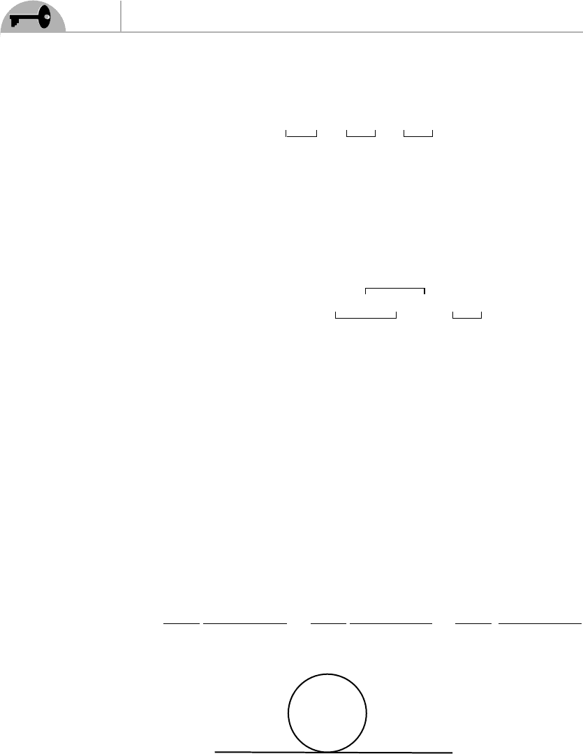
zD(x − z)D(y − z)D(z − z) (9.9)

which corresponds to Figure 9.1. The integral over three scalar propagators with

these spacetime coordinates will occur many times, so let’s have a closer look at it.

Using Eq. (9.5), we have



zD(x − z)D(y − z)D(z − z)



(2π)

−ip·(x−z)

− m

+i 



(2π)

−ik·(y−z)

− m

+i 



(2π)

−iq·(z−z)

− m

+i 

Figure 9.1 Diagram corresponding to Eq. (9.9).

CHAPTER 9 Some Explicit Calculations

181

The exponentials can be combined, and we can do the integration over z:



−ip·x−ik·y

iz·( p+k)

= e

−ip·x−ik·y

(2π)

( p + k)

= e

−ip·(x−y)

(2π)

( p + k) (9.10)

where in the last step we have set k =−p in the exponential because this is enforced

by the Dirac delta. We now can use the delta function to do trivially the integration

over k which leads us to



zD(x − z)D(y − z)D(z − z)



(2π)

−ip·(x−y)

− m

+i 

− m

+i 



(2π)

− m

+i 



(2π)

−ip·(x−y)

D( p) D( p)



(2π)

− m

+i 

(9.11)

If we Fourier transform to momentum space, we obtain





zD(x − z)D(y − z)D(z − z)





= D( p) D( p) I

(9.12)

where we have deﬁned the quadratically divergent integral

≡



(2π)

− m

+i 

(9.13)

To explicitly show the structure of the divergences arising from this integral, let us

carry out the integration. The integrand has poles at q

=±



q

+ m

∓i . With

a choice of appropriate contour, it is straightforward to show that



(2π)

− m

+i 



q

(2π)



q

+ m

(9.14)

182

Supersymmetry Demystified

Using an explicit cutoff on the magnitude of the three-momentum, we get

4π







+ m

8π





1 +



− m





− m



1 +



!

≈

8π





− m





+ m

× ﬁnite piece



(9.15)

This shows that the integral contains a quadratically divergent term that is inde-

pendent of the mass of the particle as well as a logarithmic divergence and a ﬁnite

contribution that both depend on the mass. These observations will be important

when we discuss SUSY breaking in Chapter 14.

When it comes to calculations of physical processes, the quantity of relevance

(to use in the LSZ reduction formula) is actually the amputated momentum space

propagator that is obtained from Eq. (9.12) by dropping the two propagators D( p)

associated with the external lines:





zD(x − z)D(y − z)D(z − z)





= I

(9.16)

Therefore, the amputated one-loop propagator is

( p) =−12 i λ I

(9.17)

Quadratic divergences are ubiquitous in theories with scalar ﬁelds. The beauty

of SUSY is that it rids us of these nasty divergences in a very clever manner, as we

will soon see in simple examples.

9.2 Propagators

Before doing any calculations in the Wess-Zumino model, we need the propagators

of a Majorana fermion. Since we will use Greek subscripts to indicate the compo-

nents of the Majorana spinors, these will be represented by 

instead of 

make the notation less cumbersome.

CHAPTER 9 Some Explicit Calculations

183

As for a Dirac spinor, we have

0|T





(x)

(y)



|0=



(2π)

−ik·(x−y)

αβ

(k) (9.18)

with

αβ

(k) ≡ i

(/k + m)

αβ

− m

+i 

(9.19)

However, unlike Dirac spinors, there are two additional propagators coming from

the contractions of 



and



. These propagators are identically zero for a

Dirac spinor because they contain the vacuum expectation value of the product of

a creation and an annihilation operator for the fermion and the antifermion, which

is zero because those are two distinct states. The corresponding expressions for a

Majorana fermion are not zero because it is its own antiparticle.

It is easy to work out these two extra propagators from the result in Eq. (9.18) if

we recall that for a Majorana fermion [see Eq. (4.2)],

(

)

= 

(9.20)

where the charge-conjugation operation is deﬁned as



= C 

(9.21)

and the matrix C, as given in Section 4.1, is equal to

C =



iσ

0 −iσ



(9.22)

Note that C

=−1, which implies that C

−1

=−C. We obviously also have C

−C,soC

= C

−1

. These relations will be very useful when we calculate scattering

amplitudes.

Showing the spinor indices explicitly, Eqs. (9.20) and (9.21) translate to



= C

αβ

()

(9.23)

Consider the propagator

0|T





(x)

(y)



|0 (9.24)

184

Supersymmetry Demystified

What we want to do is to rewrite this in a form similar to Eq. (9.18) using Eq. (9.23).

Obviously, we simply have to replace 

in Eq. (9.24) with C

βγ

()

, which allows

us to express the propagator (9.24) in terms of Eq. (9.18):

0|T





(x)

(y)



|0=



(2π)

−ik·(x−y)

βγ

αγ

(k)

However, this is not the most convenient form. When we will calculate diagrams,

we will want to calculate the traces of the matrices acting on the spinors, and for

this reason, it is more useful to have the index γ in the C matrix to appear in the

ﬁrst position, which we can do simply by using C

βγ

= C

γβ

, to ﬁnally get

0|T





(x)

(y)



|0=



(2π)

−ik·(x−y)

αγ

(k) C

γβ

(9.25)

This way, the matrices C

and S form a matrix product equal to SC

Following the same approach, it is easy to show that

0|T





(x)

(y)



|0=



(2π)

−ik·(x−y)

αγ

γβ

(k) (9.26)

When drawing Feynman diagrams involving Majorana spinors (and Weyl spinors

too), one has to distinguish among the three different types of fermion propagators.

This is done by drawing on the fermion lines two arrows ﬂowing in opposite

directions (either toward one another or away from one another) to represent the two

new types of propagators, Eqs. (9.25) and (9.26), in addition to the usual propagator,

Eq. (9.18), which is represented, as usual, with a single arrow. We won’t introduce

this notation for the very few calculations we will do. We will simply use the same

diagram to represent all three types of propagators. The double-arrow notation is

very useful for drawing general conclusions about the types of counterterms that

can be generated by a given lagrangian. A simple illustration of this notation for

Majorana spinors can be found in Section 1.3 of Ref. 8.

Let us note that we could, of course, carry out all the calculations using two-

component Weyl spinors instead of four-component Majorana spinors. In Ref. 13,

a detailed explanation of the Feynman rules and diagrammatic notation for Weyl

CHAPTER 9 Some Explicit Calculations

185

spinors (which also involves the double-arrow notation) is presented, as well as a

large number of detailed calculations.

The propagator of a scalar ﬁeld is, of course, the usual

0|T



A(x)A(y)



|0=



(2π)

−ik·(x−y)

(k) (9.27)

where

(k) ≡

− m

+i 

(9.28)

Note that we don’t put any label on the masses because all the particles have the

same mass.

For the rest of this chapter we will not include a label M on the Majorana spinors.

It will be understood that all spinors  will represent Majorana spinors, not Dirac

spinors.

9.3 One Point Function

As a warm-up exercise, consider the one-point function of the A ﬁeld in the Wess-

Zumino model:

|A(x)| (9.29)

This turns out to be much simpler than the zero-point (vacuum energy) calculation.

If we work to order g in the coupling constant, the calculation involves only three

simple diagrams. Despite its simplicity, this is still an interesting calculation to work

through because it will exhibit clearly the clever way in which a supersymmetric

theory takes care of the quadratic divergences.

To be explicit, the one-point function is given by

|T



A(x)



|=

0|T



A(x)e





(z)



|0

0|T (e





(z)

)|0

(9.30)

where the interaction lagrangian of the Wess-Zumino model is given by the sum of

the four terms of Eq. (8.71). Note in particular that L

I 1

is of order g

, whereas the

other three interactions are of order g.