Korb K.B., Nicholson A.E. Bayesian Artificial Intelligence

Подождите немного. Документ загружается.

3. Arcs are then checked individually for an improved MDL measure via arc

reversal.

4. Loop at Step 2.

The results achieved by this algorithm were similar to those of K2, but without

requiring a full variable ordering. Results without signiﬁcant initial information from

humans (i.e., starting from an empty partial ordering and no arcs) were not good,

however.

8.3.2 Suzuki’s MDL code for causal discovery

Joe Suzuki, in an alternative MDL implementation [273], points out that Lam and

Bacchus’s parameter encoding is not a function of the size of the data set. This

implies that the code length cannot be efﬁcient. Suzuki proposes as an alternative

MDL code for causal structures:

(8.8)

which can be added to

to get a total MDL score for the causal model. This

gives a better account of the complexity of the parameter encoding, but entirely does

away with the structural complexity of the Bayesian network! To be sure, structural

complexity is reﬂected in the number of parameters. Complexity in Bayesian net-

works corresponds to the density of connectivity and the arity of parent sets, both of

which increase the number of parameters required for CPTs. Nevertheless, that is

by no means the whole story to network complexity, as there is complexity already

in some topologies over others entirely independent of parameterization, as we shall

see below in

8.5.1.1.

8.4 Metric pattern discovery

From Chapter 6 we know that dags within a single pattern are Markov equivalent.

That is, two models sharing the same skeleton and v-structures can be parameterized

to identical maximum likelihoods and so apparently cannot be distinguished given

only observational data. This has suggested to many that the real object of metric-

based causal discovery should be patterns rather than the dags being coded for by

Lam and Bacchus. This is a possible interpretation of Suzuki’s approach of ignoring

the dag structure entirely. And some pursuing Bayesian metrics have also adopted

this idea (e.g., [240, 46]). The result is a form of metric discovery that explicitly

mimics the constraint-based approach, in that both aim strictly at causal patterns.

The most common approach to ﬁnding an uninformed prior probability over

the model space — that is, a general-purpose probability reﬂecting no prior domain

knowledge — is to use a uniform distribution over the models. This is exactly what

Cooper and Herskovits did, in fact, when assigning the prior

to all dag

structures. Pattern discovery assigns a uniform prior over the Markov equivalence

classes of dags (patterns), rather than the dags themselves. The reason adopted is

that if there is no empirical basis for distinguishing between the constituent dags,

then empirical considerations begin with the patterns themselves. So, considerations

before the empirical — prior considerations — should not bias matters; we should

let the empirical data decide what pattern is best. And the only way to do that is to

assign a uniform prior over patterns.

We believe that such reasoning is in error. The goal of causal discovery is to

ﬁnd the best causal model, not the best pattern. It is a general and well-accepted

principle in Bayesian inference that our prior expectations about the world should not

be limited by what our measuring apparatus is capable of recording (see, e.g., [173]).

For example, if we thought that all four possible outcomes of a double toss of a coin

were equally likely, we would hardly revise our opinion simply because we were

told in advance that the results would be reported to us only as “Two heads” or “Not

two heads.” But something like that is being proposed here: since our measuring

apparatus (observational data) cannot distinguish between dags within a pattern, we

should consider only the patterns themselves.

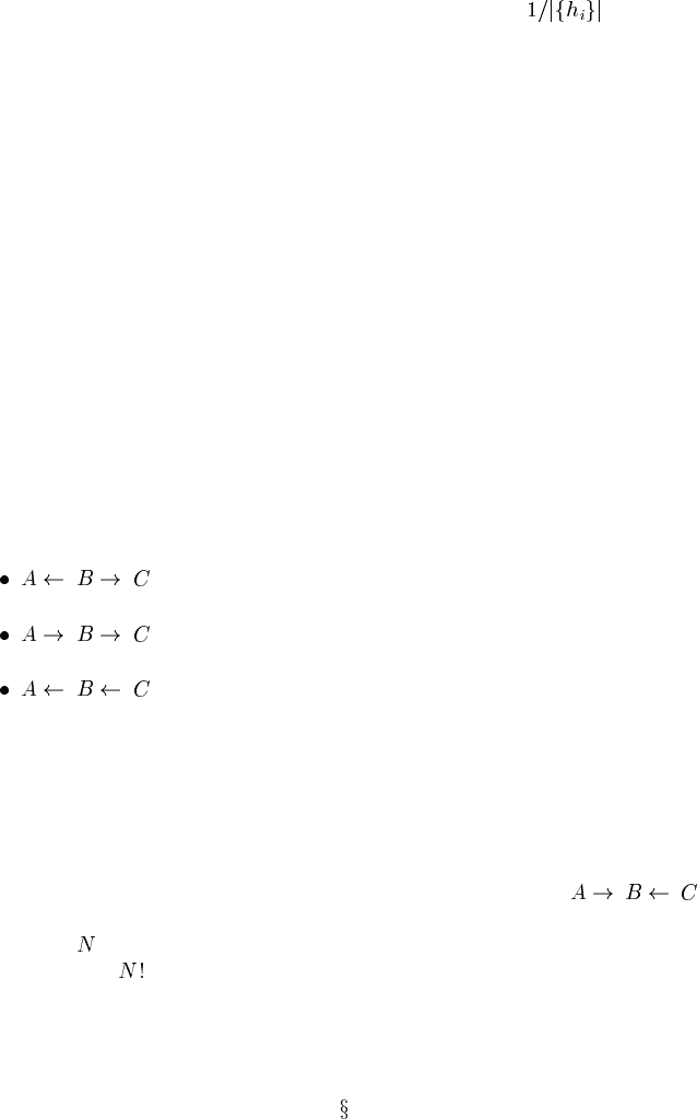
The relevant point, however, is that the distinct dags within a pattern have quite

distinct implications about causal structure. Thus, all of

are in the same pattern, but they have entirely different implications about the effect

of causal interventions. Even if we are restricted to observational data, we are not in

principle restricted to observational data. The limitation, if it exists, is very like the

restriction to a two-state description of the outcome of a double coin toss: it is one

that can be removed. To put it another way: the pattern of three dags above can be

realized in at least those three different ways; the alternative pattern of

can be realized only by that single dag. Indeed, the number of dags making up a

pattern over

variables ranges from a pattern with one dag (patterns with no arcs)

to a pattern with

dags (fully connected patterns). If we have no prior reason to

prefer one dag over another in representing causal structure, then by logical necessity

we do have a prior reason to prefer patterns with more dags over those with fewer.

Those advocating pattern discovery need to explain why one dag is superior to

another and so should receive a greater prior probability. We, in fact, shall ﬁnd prior

reasons to prefer some dags over others (

8.5.1.1), but not in a way supporting a

uniform distribution over patterns.

8.5 CaMML: Causal discovery via MML

We shall now present our own method for automated causal discovery, implemented

in the program CaMML, which was developed in large measure by Chris Wallace,

the inventor of MML [290]. First we present the MML metric for linear models.

Although we dealt with linear models in Chapter 6, motivating constraint-based

learning with them, we ﬁnd it easier to introduce the causal MML codes with lin-

ear models initially. In the next section we present a stochastic sampling approach

to search for MML, in much more detail than any other search algorithm. We do

so because the search is interestingly different from other causal search algorithms,

but also because the search affords an important simpliﬁcation to the MML causal

structure code. Finally, only at the end of that section, we present the MML code

for discrete models. Because of the nature of the search, that code can be presented

as a simple modiﬁcation of the Cooper and Herskovits probability distribution over

discrete causal models.

Most of what was said in introducing MDL applies directly to MML. In particular,

both methods perform model selection by trading off model complexity with ﬁt to the

data. The main conceptual difference is that MML is explicitly Bayesian and it takes

the prior distribution implied by the MML code seriously, as a genuine probability

distribution.

One implication of this is that if there is a given prior probability distribution for

the problem at hand, then the correct MML procedure is to encode that prior proba-

bility distribution directly, for example, with a Huffman code (see [60, Chapter 5] for

an introduction to coding theory). The standard practice to be seen in the literature is

for an MML (or, MDL) paper to start off with a code that makes sense for communi-

cating messages between two parties who are both quite ignorant of what messages

are likely. The simplest messages (the simplest models) are given short codes and

messages communicating more complex models are typically composites of them,

and so are longer in an effectively computable way. That standard practice makes

perfect sense (and, we shall follow it here) — unless a speciﬁc prior distribution is

available, which implies something less than total prior ignorance about the problem.

In any such case, considerations of efﬁciency, and the relation between code length

and probability in (8.4), require the direct Huffman encoding (or similar). In short,

MML is genuinely a Bayesian method of inference.

8.5.1 An MML code for causal structures

We shall begin by presenting an MML code for causal dag structures. We assume in

developing this code no more than was assumed for the MDL code above (indeed,

somewhat less). In particular, we assume that the number of variables is known. The

MML metric for the causal structure

has to be an efﬁcient code for a dag with

variables. can be communicated by:

First, specify a total ordering. This takes bits.

Next, specify all arcs between pairs of variables. If we assume an arc density

= 0.5 (i.e., for a random pair of variables a 50:50 chance of an arc)

, we need

one bit per pair, for the total number of bits:

However, this allows multiple ways to specify the dag if there is more than

one total ordering consistent with it (which are known as linear extensions of

the dag). Hence, this code is inefﬁcient. Rather than correct the code, we can

simply compensate by reducing the estimated code length by

,where

is the number of linear extensions of the dag. (Remember: we are not actually

in the business of communication, but only of computing how long efﬁcient

communications would be!)

Hence,

(8.9)

8.5.1.1 Totally ordered models (TOMs)

Before continuing with the MML code, we consider somewhat further the question

of linear extensions. MML is, on principle, constrained by the Shannon efﬁciency

requirement to count linear extensions and reduce the code length by the redundant

amount. This is equivalent to increasing the prior probability for dags with a greater

number of linear extensions over an otherwise similar dag with fewer linear exten-

sions. Since these will often be dags within the same Markov equivalence class

(pattern), this is a point of some interest. Consider the two dags of Figure 8.2: the

chain has only one linear extension — the total ordering

— while the

common cause structure has two — namely,

and .And

both dags are Markov equivalent.

CBA

(a)

(b)

FIGURE 8.2

A Markov equivalent: (a) chain; (b) common cause.

We shall remove this assumption below in 8.6.3.

The most common approach by those pursuing Bayesian metrics for causal dis-

covery thus far has been to assume that dags within Markov equivalence classes

are inherently indistinguishable, and to apply a uniform prior probability over all

of them; see, for example, Madigan et al. [177]. Again, according to Heckerman

and Geiger [103], equal scores for Markov equivalent causal structures will often be

appropriate, even though the different dag structures can be distinguished under the

causal interpretation.

Note that we are not here referring to a uniform prior over patterns, which we con-

sidered in

8.4, but a uniform prior within patterns. Nonetheless, the considerations

turn out to be analogous. The kind of indistinguishability that has been justiﬁed for

causal structures within a single Markov equivalence class is observational indistin-

guishability. The tendency to interpret this as in-principle indistinguishability is not

justiﬁed. After all, the distinguishability under the causal interpretation is clear: a

causal intervention on

in Figure 8.2 will inﬂuence in the chain but not in the

common causal structure. Even if we are limited to observational data, the differ-

ences between the chain and the common cause structure will become manifest if we

expand the scope of our observations. For example, if we include a new parent of

a new v-structure will be introduced only if

is participating in the common causal

structure, resulting in the augmented dags falling into distinct Markov equivalence

classes.

We can develop our reasoning to treat linear extensions. A totally ordered model,

or TOM, is a dag together with one of its linear extensions. It is a plausible view of

causal structures that they are, at bottom, TOMs. The dags represent causal processes

(chains) linking together events which take place, in any given instance, at particular

times, or during particular time intervals. All of the events are ordered by time.

When we adopt a dag, without a total ordering, to represent a causal process, we are

representing our ignorance about the underlying causal story by allowing multiple,

consistent TOMs to be entertained. Our ignorance is not in-principle ignorance: as

our causal understanding grows, new variables will be identiﬁed and placed within

it. It is entirely possible that in the end we shall be left with only one possible linear

extension for our original problem. Hence, the more TOMs (linear extensions) that

are compatible with the original dag we consider, the more possible ways there are

for the dag to be realized and, thus, the greater the prior probability of its being true.

In short, not only is it correct MML coding practice to adjust for the number of

linear extensions in estimating a causal model’s code length, it is also the correct

Bayesian interpretation of causal inference.

This subsection might well appear to be an unimportant aside to the reader, espe-

cially in view of this fact mentioned previously in

8.2.1: counting linear extensions

is exponential in practice [32]. In consequence, the MML code presented so far does

not directly translate into a tractable algorithm for scoring causal models. Indeed, its

direct implementation in a greedy search was never applied to problems with more

than ten variables for that reason [293]. However, TOMs ﬁgure directly in the sam-

pling solution of the search and MML scoring problem, in section

8.6 below.

8.5.2 An MML metric for linear models

So, we return to developing the MML metric. We have seen the MML metric for

causal structure; now we need to extend it to parameters given structure and to data

given both parameters and structure. We do this now for linear models; we de-

velop the MML metric for discrete models only after describing CaMML’s stochas-

tic search in

8.6, since the discrete metric takes advantage of an aspect of the search.

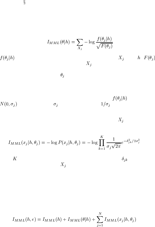
The parameter code. Following Wallace and Freeman [292], the message length

for encoding the linear parameters is

(8.10)

is the prior density function over the parameters for given . is

the Fisher information for the parameters to

. It is the Fisher information which

controls the precision of the parameter estimation. In effect, it is being used to dis-

cretize the parameter space for

, with cells being smaller (parameters being more

precisely estimated) when the information afforded by the data is larger. (For details

see [292].)

Wallace et al. [293] describe an approximation to (8.10), using the standard as-

sumptions of parameter independence and the prior density

being the normal

, with the prior for being proportional to .

The data code. The code for the sample values at variable

given both the pa-

rameters and dag is, for i.i.d. samples,

(8.11)

where

is the number of joint observations in the sample and is the difference

between the observed value of

and its linear prediction. Note that this is just a

coding version of the Normal density function, which is the standard modeling as-

sumption for representing unpredicted variation in a linear dependent variable.

The MML linear causal model code. Combining all of the pieces, we have the

total MML score for a linear causal model being:

(8.12)

8.6 CaMML stochastic search

Having the MML metric for linear causal models in hand, we can reconsider the

question of how to search the space of causal models. Rather than apply a greedy

search, or some variant such as beam search, we have implemented two stochastic

searches: a genetic algorithm search [201] and a Metropolis sampling process [294].

8.6.1 Genetic algorithm (GA) search

The CaMML genetic algorithm searches the dag space; that is, the “chromosomes”

in the population are the causal model dags themselves. The algorithm simulates

some of the aspects of evolution, tending to produce better dags over time — i.e.,

those with a lower MML score. The best dags, as reported by the MML metric, are

allowed to reproduce. Offspring for the next generation are produced by swapping a

subgraph from one parent into the graph of the other parent and then applying muta-

tions in the form of arc deletions, additions and reversals. A minimal repair is done

to correct any introduced cycles or reconnect any dangling arcs. Genetic algorithms

frequently suffer from getting trapped in local minima, and ours was no exception.

In order to avoid this, we introduced a temperature parameter (as in simulated an-

nealing) to encourage a more wide-ranging search early in the process. None of this

addresses the problem of counting linear extensions for the MML metric itself. We

handled that by an approximative estimation technique based upon that of Karzanov

and Khachiyan [141]. For more details about our genetic algorithm see [201]. Al-

though the GA search performs well, here we shall concentrate upon the Metropolis

sampling approach, as it offers a more telling solution to the problem of counting

linear extensions.

8.6.2 Metropolis search

Metropolis sampling allows us to approximate the posterior probability distribution

over the space of TOMs by a sampling process. From that process we can estimate

probabilities for dags. The process works by the probability measure providing a

kind of pressure on the sampling process, ensuring that over the long run models

are visited with a frequency approximating their probabilities [189, 176]. This is a

type of Markov Chain Monte Carlo (MCMC) search, meaning that the probabilis-

tically selected sequence of sampled models forms a Markov Chain (the probability

of reaching any particular model depends only upon what model is currently being

sampled and not on the sampling history). The probabilities for our CaMML im-

plementation are, of course, derived from the MML metric. Since the models being

sampled are TOMs, rather than dags, the MML metric is computed for TOMs only

at each step. Hence there is no (direct) problem with counting linear extensions.

Since we are searching in the space of TOMs, we need an adjustment of

(8.9) to reﬂect the change. This is, very conveniently, simply to drop the term requir-

ing us to count linear extensions. Hence,

(8.13)

with

now ranging over TOMs rather than dags.

ALGORITHM 8.2

CaMML Metropolis Algorithm

1. First, an initial TOM is selected at random. Call this

2. Uniformly randomly choose between the following possible changes to the

current model

producing :

(a) Temporal order change: Swap the order of two neighboring nodes. (If

there is an arc between them, it reverses direction.)

(b) Skeletal change: Add (or delete) an arc between two randomly selected

nodes.

arcs between the ﬁrst two nodes and the last (in the temporal order).

(Double changes are not necessary for the Metropolis algorithm to work,

but are included to help accelerate the sampling process.)

3. Accept

as the new if ; otherwise retain .

where

and is a uniform random variate in the interval .

4. Count the current visit to

5. Loop at 2 (until an input number of samples has been completed).

This Monte Carlo process meets the sufﬁcient conditions for the Metropolis algo-

rithm to apply, viz., the number of possible transitions from each TOM is constant,

and every transition is reversible [189]. The process will therefore visit every TOM

with a frequency proportional to its joint probability with the data, and hence pro-

portional to its MML posterior.

We are not directly interested in the posterior probabilities of individual TOMs,

but instead in the probabilities of sets of TOMs which are sufﬁciently similar to be

grouped together and represented by a single MML model. (We expand on this

grouping process in

8.6.4.) The total posterior given by MML to the representative

is the sum of the posteriors of the member TOMs. We therefore do not count visits

to individual TOMs, but visits to MML models.

Whenever the MML model is changed by a step, the skeleton and maximized

likelihood is found. Recall from Chapter 6 that all Markov equivalent models share

these properties. We then attempt to count visits to (skeleton-likelihood) pairs. In

a problem with many variables, there will be far too many such pairs to allow for

exact counting. So, we form a hash index from the (skeleton-likelihood) pair into a

65536-entry table, using different random keys for each possible arc. Distinct MML

models are therefore unlikely to yield the same hash indices, which would throw

off the estimated posterior probability. To be even safer, we actually maintain two

distinct hash tables with distinct random keys and use the lesser count at the end of

the sampling process to estimate posterior probabilities. That estimate is simply the

ﬁnal count, divided by the number of sampling steps.

Note that the process of ﬁnding a representative MML model is used only to up-

date the hash table count and does not inﬂuence the sampling process by changing

the current TOM from which it is derived.

During sampling, the program accumulates a list of up to 50 MML models, being

those with the highest estimated posterior. Each retained MML model is represented

by its highest-posterior dag. The dag posterior is estimated using a further two tables

for which the hash indices are calculated from “dag signatures.” These signatures are

formed like the MML model signatures, but use a different matrix of pseudo-random

constants and do not use likelihoods. This matrix is not symmetrical, allowing the

dag signature to capture arc directions as well as skeletons. The dag counts are, of

course, updated after each sampling step.

At the end of the sampling, the selected models are displayed. For each retained

MML model CaMML displays: its posterior, the posterior of the highest-posterior

dag, the arcs and estimated parameters. It also reports the weighted frequency of

directed arcs across the retained models. For more details of the sampling process

see [294].

8.6.3 Prior constraints

TETRAD II allows prior variable orderings to be speciﬁed, by grouping variables

in tiers. Variables in earlier tiers are constrained during search not to be effects of

variables in later tiers. Variables within a tier can be discovered to exist in causal

chains in any (non-cyclic) order. Of course, by having as many tiers as variables,

one can impose a total ordering upon the variables.

An interesting alternative method of specifying prior probability is that adopted

by Heckerman and Geiger [103] for their Bayesian BDe and BGe metrics. They

have the user generate a “best guess” causal model in the beginning. Their prior

probability metric then rewards models which are closer to this best guess model (in

edit distance terms of arc deletions, additions and reversals).

CaMML has a more ﬂexible system of prior constraints. For each pair of variables

the user can specify a prior probability for the existence of a particular directed arc

between them. Any arc probabilities left unspeciﬁed are assigned the default

. In the structure code, instead of coding each possible arc, or absence of an

arc, as one bit, as in Equations (8.9) and (8.13), those equations are modiﬁed to

reﬂect the prior probability

for each possible directed arc . In particular, for each

arc in a model CaMML adds

bits and for each missing possible arc it adds

. Thus we get the following MML structural metric:

(8.14)

where

indexes the arcs in a TOM and indexes the possible arcs that are absent in

the TOM.

By assigning a zero prior probability to sets of directed arcs, one can force all

causal relations between two non-overlapping sets of variables to hold in a ﬁxed

direction — in other words, tiers of variables can be identiﬁed, as with TETRAD

II. Similarly, CaMML’s soft prior constraints on arcs can be made to mimic the edit

distance metric of Heckerman and Geiger. Much prior expert “knowledge” is not

knowledge at all, but opinion. This relevant human expertise in general is valuable,

opinion or not. Hence, the soft constraint of selecting prior probabilities for directed

arcs near, but not identical to, 0 or 1 is valuable, and it provides options which neither

the Heckerman and Geiger nor TETRAD regimes allow.

8.6.4 MML models

We now describe the grouping of TOMs into the MML model for which visit counts

are kept. First, TOMs which differ only in the order of the variables, but with the

same skeleton and arc directions, are clearly indistinguishable given the data, and so

will be grouped. All TOMs in the group are linear extensions of the same dag.

Suppose two TOMs

and differ only in that contains an arc not present

. If the magnitude of this causal effect is sufﬁciently small, the MML code

length may be reduced by grouping

and together, and using the simpler

as the representative model. This can shorten the total message, because the prior

probability of the group is the sum of the priors of

and . The data may be

encoded in a longer message with

rather than with the small effect model ,but

if the coefﬁcient of the extra arc is small, that increase in the length of the data part

of the message may well be less than the reduction in ﬁrst part encoding the model.

CaMML performs an approximate check whether neighboring TOMs should be

grouped together on this basis. The TOM within such a group without small effects

is chosen as its representative model and used to compute parameters and data length.

It may be thought that deleting small effect arcs is an unimportant reﬁnement of

the MML process. Others using stochastic sampling for causal discovery have not

employed it (e.g., [177]). However, typically for a TOM

there will be about

other TOMs differing from it only by the addition of a small effect. The total joint

probability (and hence posterior probability) of all such TOMs may therefore be

about

times that of A, where is the data set size. Unless is greater than

, there may be more total posterior probability over these small effect TOMs than

itself; so inclusion of them in the set represented by adds signiﬁcantly to the

posterior probability of the set. Indeed, in a large model space the search may never

actually sample the representative model. Of course, in the limit it must do so, but

lacking inﬁnite patience, we prefer to group models.