Kline R.B. Principles and Practice of Structural Equation Modeling
Подождите немного. Документ загружается.

374 Suggested Answers to Exercises
7. Both measurement errors and disturbances are represented as latent variables in some SEM
computer tools, and their variances are typically free parameters that require a statistical
estimate. Both represent residual (unexplained) variance, including that due to all omitted
causes and score unreliability, too. The term disturbance has its roots in path analysis, and
disturbances are associated with endogenous variables in structural models. In path models,
all endogenous variables are observed variables, but some factors in structural regression
models are endogenous, and each of the latter variables has its own disturbance. Measure-
ment errors are associated exclusively with observed variables, specifically, with indicators
in a measurement model.
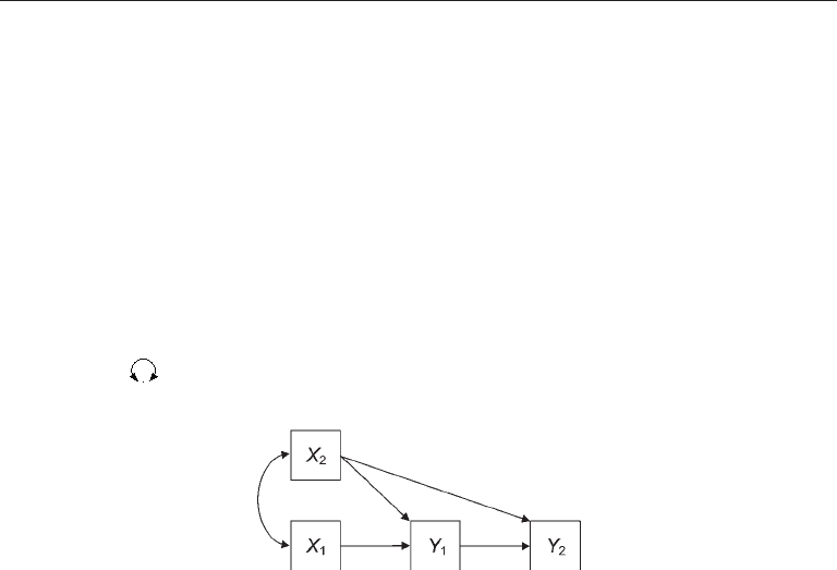
8. Presented next is a basic path model shown without the symbols for disturbances (e.g., D
1
for Y
1
, D
2
for Y
2
) and variances of measured (X
1
, X
2
) or unmeasured (D
1
, D
2
) exogenous
variables (
). Variable X
2
is the covariate, and estimation of the effects of X
1
are corrected
for its covariance with the covariate:
9. Sample size has nothing to do with the number of observations, the number of model param-
eters, df
M
, or model identification. As in basically all statistical analyses, sample size in SEM
affects the precision of the results in the form of standard errors (larger N, smaller standard
errors, and vice versa). Large samples are generally required in SEM for acceptable precision,
and some special methods may require even larger samples still. A larger sample size can
also prevent some technical problems, such as iteration failure, that can occur in computer
analyses.
ChaPter 6
1. Path models: Parameters of path models include (a) direct effects on endogenous variables
from other endogenous variables or measured exogenous variables (i.e., path coefficients);
and (b) variances and covariances of measured exogenous variables and disturbances.
CFA models: Parameters of CFA models include (a) direct effects on indicators from factors
(i.e., factor loadings); and (b) variances and covariances of the factors and measurement
errors.
SR models: Parameters of SR models include (a) direct effects on endogenous variables, includ-
ing factor loadings of indicators in the measurement model and direct effects on endogenous
factors in the structural model; and (b) variances and covariances of exogenous variables,
including measurement errors, disturbances, and exogenous factors.
2. Factor B and indicator X
3
of Figure 6.4(c) would have the same scale only if the factor explains
100% of the variance of the indicator (unlikely). Otherwise, the scale of B is related to the
Suggested Answers to Exercises 375
scale of the explained variance X
3
, not typically the total (observed) variance of this indica-
tor.
3. The number of observations for both CFA models in Figure 6.1 is 6(7)/2 = 21. The breakdown
of parameters for both models is listed next. There are 13 parameters for each model, so
df
M
= 8 for both factor models:
Exogenous variables
Model Direct effects on indicators Variances Covariances Total
Figure 6.1(a) A → X
2
B → X
5
A, B A B 13
A → X
3
B → X
6
E
1
–E
6
Figure 6.1(b) A → X
1
B → X
4
E
1
–E
6
A B 13
A → X
2
B → X
5
A → X
3
B → X
6
4. With four observed variables, there are 4(5)/2 = 10 observations available to estimate the
parameters of the nonrecursive path model in Figure 6.3. The parameters of this model
include these five direct effects
X
1
→ Y
1
, X
1
→ Y
2
, X
2
→ Y
2
, Y
1
→ Y
2
, and Y
2
→ Y
1
and four variances (of X
1
, X
2
, D
1
, and D
2
) and two covariances (of X
1
X
2
and D
1
D
2
)
of exogenous variables for a total of 11, so df
M
= –1. This model fails the order condition
because there are no excluded variables for Y
2
(i.e., the equation for this endogenous variable
is underidentified). The same equation also fails the rank condition because the rank of the
reduced system matrix for Y
2
is zero:
X
1
X
2
Y
1
Y
2
Y
1
1 0 1 1
→
Y
2
1 1 1 1
→
→
Rank = 0
5. After the path X
3
→ Y
1
and the corresponding unanalyzed associations are added to the
model in Figure 6.3, there are 5(6)/2 = 15 observations available to estimate the parameters
of the respecified model, including five variances (of X
1
–X
3
, D
1
, and D
2
), four covariances (of
X
1
X
2
, X
1
X
3
, X
2
X
3
, and D
1
D
2
), and these six direct effects
X
1
→ Y
1
, X
1
→ Y
2
, X
2
→ Y
2
, X
3
→ Y
1
, Y
1
→ Y
2
, and Y
2
→ Y
1
for a total of 15 free parameters, so df
M
= 0. There is at least one variable omitted from the
equation of each endogenous variable (X
2
for Y
1
, X
3
for Y
2
), so the order condition is satisfied.
Evaluation of the sufficient rank condition for the respecified model is outlined next:
Evaluation for Y
1
:
X
1
X
2
X
3
Y
1
Y
2
→
Y
1
1 0 1 1 1
Y
2
1 1 0 1 1
→
1
→
Rank = 1
376 Suggested Answers to Exercises
Evaluation for Y
2
:
X
1
X
2
X
3
Y
1
Y
2
Y
1
1 0 1 1 1
→
Y
2
1 1 0 1 1
→
1
→
Rank = 1
Because the rank of the equation for each endogenous variable equals the minimum required
value, or 1, the sufficient rank condition is satisfied. Thus, the respecified model is just-
identified.
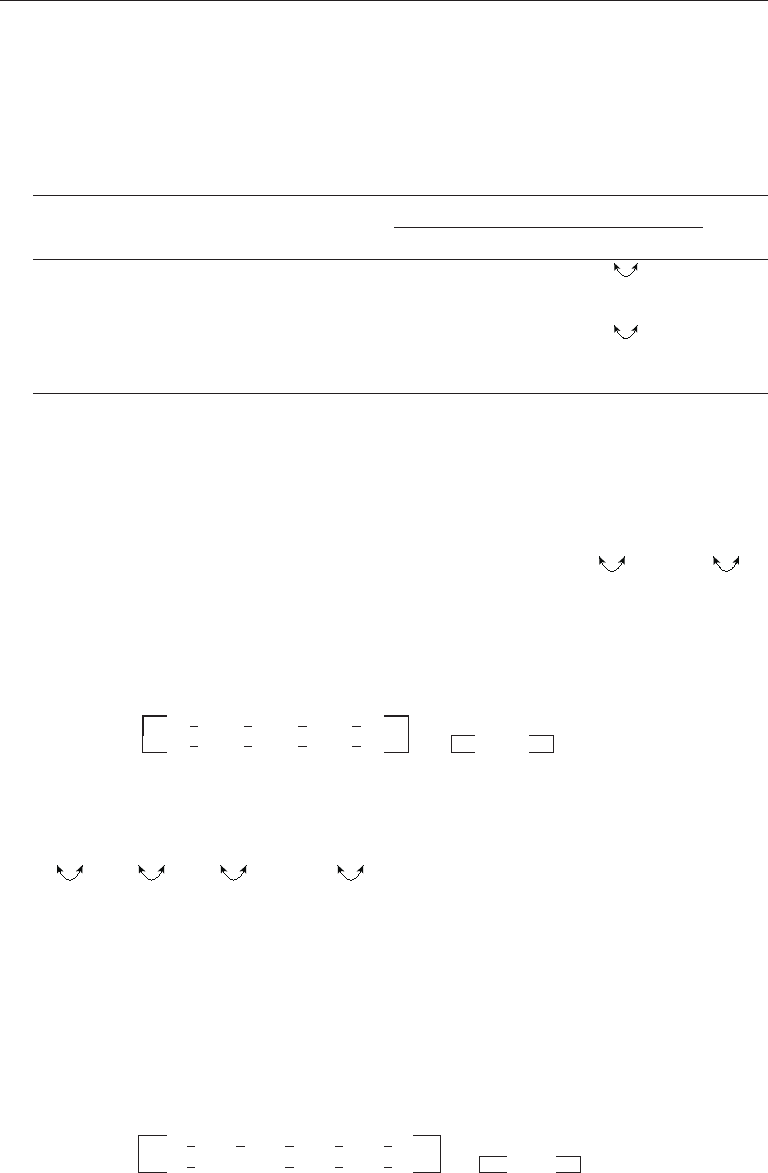
6. Yes, the model in Figure 6.5(f) with complex indicator X
3
but with the error correlation
E
X
3
E
X
5
is identified because this respecified model satisfies Rule 6.8 in Table 6.2. Spe-
cifically, the respecified model satisfies Rule 6.7 (and by implication Rule 6.6; see Table 6.1)
and there is at least one singly loading indicator on each of factor A and B with which the
complex indicator X
3
does not share an error correlation (e.g., X
2
← A, X
4
← B). For the sec-
ond part of this question, we are now working with the respecified model presented next:
Adding the error correlation E
X
3
E
X
4
to this respecified model would result in a non-
identified model that violates Rule 6.8 because there would be no indicator of B that does not
share an error correlation with the complex indicator X
3
. It would be possible to add either
E
X
1
E
X
3
or E
X
2
E
X
3
to the respecified model (i.e., each of the resulting models would
be identified), but not both. This is because the respecified model but with both error cor-
relations just mentioned would violate Rule 6.8 in that there would be no indicator of A that
shares no error correlation with X
3
.
7. The virtual absence of the path X
2
→ Y
2
alters the system matrix for the first block of endog-
enous variables in Figure 6.2(b). This consequence is outlined next, starting with the matrix
for the model in the figure without the path X
2
→ Y
2
(the rank for Y
1
’s equation is zero):
X
1
X
2
Y
1
Y
2
→
Y
1
1 0 1 1
Y
2
0 0 1 1
→
0
→
Rank = 0
8. For the SR model in Figure 6.6(a), df
M
= 7, so it seems as though there is “room” for more
effects, but let’s apply the two-step rule: the measurement portion expressed as a CFA model
with the error correlations E
X
1
E
Y
1
, and E
X
2
E
Y
2
would be identical to the measure-
Suggested Answers to Exercises 377
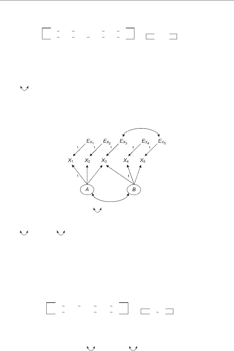
ment model in Figure 6.5(e), which is identified. The structural model after adding the dis-
turbance correlation D
B
D
C
is presented next:
This structural model is nonrecursive with all possible disturbance correlations. The order
condition is satisfied because there is one variable omitted from the equation of every
endogenous variable (A for B, B for C). The sufficient rank condition is also satisfied:
Evaluation for B:
A B C
→
B
1
1 0
C
0
1 1
→
1
→
Rank = 1
Evaluation for C:
A B C
B
1 1
0
→
C
0
1 1
→
1
→
Rank = 1
Therefore, the structural part of the respecified CFA model is identified. Because both the
measurement and structural models are identified, the respecified SR model is identified,
too.
ChaPter 7
1. Proportions of explained variance for the model in Figure 7.1:
Endogenous variable
2
s m c
R
Teacher Burnout 1 – (68.137/9.7697
2
) = .286
Teacher–Pupil Interactions 1 – (19.342/5.0000
2
) = .226
School Experience 1 – (7.907/3.7178
2
) = .428
Somatic Status 1 – (13.073/5.2714
2
) = .530
2. Sobel test for the model in Figure 7.1(a) of the unstandardized indirect effect of school sup-
port on student school experience through teacher-pupil interactions:
z = (.097 × .486)/
2222
.486 (.046 ) .097 (.055 )+
= 2.051
Thus, this indirect effect is statistically significant at the .05 level but not at the .01 level.
However, this result may not be accurate because the sample size is not large.

378 Suggested Answers to Exercises
3. Unstandardized total indirect effect of school support on school experience for the model
in Figure 7.1(a):
(.097 × .486) + (–.384 × .142 × .486) = .021
This value matches within slight rounding error the corresponding entry in Table 7.3 for this
unstandardized total indirect effect, or .020.
4. I used the student version of LISREL 8.8 to conduct this analysis and the next. For the
respecified model with the direct effect from school support to school experience, df
M
= 6.
The unstandardized path coefficient for this new direct effect is –.018, its estimated standard
error is .026, z = –.696, and the standardized coefficient is –.052. The new direct effect is not
statistically significant (z = –.696), but power is low, and the magnitude of this new effect
in standardized terms is not large. These results are consistent with the hypothesis of pure
mediation. The value of the test statistic from this analysis, or –.696, matches within round-
ing that of the standardized residual for the variables school and school experience in the
original model, or –.695 (see Table 7.3). In this case, both statistics test the effect of adding
a direct effect between these two variables to the original model. In the revised model with
the path from school support to school experience,
2
s m c
R
= .431, which is only slightly greater
than the corresponding statistic in the original model without this path, or
2
s m c
R
= .428.
5. For the respecified model, df
M
= 8 because just a single path coefficient is calculated for the
two equality-constrained direct effects. In the unstandardized solution, the path coefficient
for both direct effects is –.150. However, in the standardized solution, the coefficients for the
direct effects of school support and coercive control on teacher burnout are, respectively,
–.161 and –.127. Recall that equality constraints generally hold in the unstandardized solu-
tion only in default ML estimation.
6. A corrected normal theory method requires the analysis of a raw data file, not a matrix sum-
mary of the data.
7. This exercise concerned whether you could reproduce the parameter estimates in Table 7.7
for the model in Figure 7.2 and the data in Table 7.6.
8. A disturbance correlation in a path model estimates the residual (partial) correlation between
a pair of endogenous variables controlling for their common measured causes. In this case,
the sign of the residual correlation (.38) is positive, which indicates that shared unmeasured
(omitted) causes affect these two endogenous variables in the same direction. For exam-
ple, whatever omitted cause increases one endogenous variable also tends to increase the
other endogenous variable, and vice versa. This makes sense because the sample correlation
between this pair of endogenous variables is positive (.41). However, the residual correlation
(.38) is nearly as large as the observed correlation (.41). This means that the explanatory
power of the model without the disturbance correlation for this pair of endogenous variables
is relatively low.

Suggested Answers to Exercises 379
ChaPter 8
1. The largest correlation residual in Table 7.5, or .103, is for the coercive control and school
experience variables. Because the original model contains only indirect effects between
these two variables, an obvious respecification is to add a direct effect from coercive control
to school experience. For this revised model, EQS reported these values of the following fit
statistics:
2
M
χ
(6) = 1.464, p = .962, RMSEA = 0, GFI = .996, CFI = 1.000, and SRMR = .018. The
program was unable to calculate a confidence interval based on the RMSEA, perhaps because
the fit of this revised model is close to perfect. None of the correlation residuals exceed .10
in absolute value:
Variable 1 2 3 4 5 6
1. Coercive Control 0
2. Teacher Burnout 0 0
3. School Support 0 0 0
4. Teacher-Pupil 0 0 0 0
5. School Experience 0 .035 –.028 0 0
6. Somatic Status –.054 –.028 .021 0 .020 0
For the new path from coercive control to school experience in the revised model, the
unstandardized path coefficient, standard error, z statistic, and standardized coefficient are,
respectively, .055, .035, 1.568, and .123. The unstandardized path coefficient is not statisti-
cally significant, but power is low. The proportion of explained variance for the school expe-
rience variable in the revised model is
2
smc
R
= .441, which, as expected, is somewhat greater
than the value in the original model, or
2
smc
R
= .428 (see Exercise 1 for Chapter 7). Based
on these results for the respecified model, overall fit is acceptable, but this revised model is
hardly “proved.”
2. For the respecified Roth et al. path model with a direct effect from fitness to stress, EQS
reported values of the following fit statistics:
2
M
χ
(4) = 5.921, p = .205, RMSEA = .036 (0–.092),
GFI = .994, CFI = .988, and SRMR = .034. None of the absolute correlation residuals exceed
.10:
Variable 1 2 3 4 5
1. Exercise 0
2. Hardiness 0 0
3. Fitness 0 .082 0
4. Stress –.012 –.009 –.018 .004
5. Illness .029 –.095 –.006 .006 .003
3. There is only a 15.3% chance of rejecting a false model for this analysis with 109 cases, given
the other assumptions stated in Table 8.7. The minimum sample size required for a minimum
of power of .80 for the test of the close-fit hypothesis is about 1,075 cases. There is only a
9.6% chance of detecting a model with close approximate fit for this analysis. The minimum
sample size needed for power = .80 for the test of the not-close-fit hypothesis is about 960
cases.
4. For the model in Figure 8.3(a), df
M
= 5, which implies 10 free parameters:
AIC
Fig 8.3(a)
= 40.402 + 2 (10) = 60.402
380 Suggested Answers to Exercises
For the model in Figure 8.3(b), df
M
= 3, which implies 12 free parameters:
AIC
Fig 8.3(b)
= 3.238 + 2 (12) = 27.238
5. These minimum sample sizes needed for power = .80 for the test of each null hypothesis
listed next are from Table 4 of MacCallum et al. (1996, p. 144):
df
M
df
M
H
0
2 6 10 14 20 25 30 40
Close fit 3,488 1,238 782 585 435 363 314 252
Not close fit 2,382 1,069 750 598 474 411 366 307
These results make clear the reality that large samples are required for adequate statistical
power when there are few model degrees of freedom.
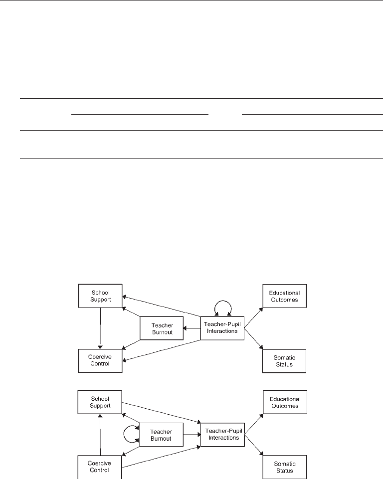
6. Several different equivalent models could be generated from Figure 7.1, but the real test is
whether a candidate equivalent model has the same values of fit statistics when fitted to the
same data as the original model. Presented next are two equivalent versions of Figure 7.1.
Your models may not exactly match these two models, but all equivalent versions will obtain
the same values of all fit statistics (e.g.,
2
M
χ
(7) = 3.895, GFI = .989, etc.):
7. The two models for this problem are not equivalent because the variables fitness and stress
in Figure 8.1 do not have common causes, which violates a requirement of Rule 8.2 of the
Lee–Hershberger replacing rules that a direct path between two endogenous variables can be
reversed if those variables have the same causes.
8. For the Roth et al. model:
CFI = 1 – [(11.078 – 5)]/[(165.499 – 10)] = 1 – (6.078/155.499) = .961

Suggested Answers to Exercises 381
For the Sava model:
CFI = 1.000 because
2
M
χ
= 3.895 < df
M
= 7
ChaPter 9
1. Values of cross-factor structure coefficients are calculated as follows:
Indicator Simultaneous Indicator Sequential
HM .497 (.557) = .277 GC .503 (.557) = .280
NR .807 (.557) = .449 Tr .726 (.557) = .404
WO .808 (.557) = .450 SM .656 (.557) = .365
MA .588 (.557) = .328
PS .782 (.557) = .436
2. Listed here are values of standardized residuals for this analysis computed by the student
version of LISREL. Absolute values > 1.96 are statistically significant at the .05 level:
Indicator HM NR WO GC Tr SM MA PS
HM 0
NR –.555 0
WO –2.642 4.472 0
GC 1.141 –2.237 –1.280 0
Tr 2.141 –1.463 –.959 .438 0
SM 3.769 –.111 –.350 –.758 –.259 0
MA 3.791 1.166 .741 .326 –.240 .688 0
PS 3.247 –1.816 .538 .971 .763 –.141 –1.647 0
3. Sum of unstandardized factor loadings:
(1.000 + 1.445 + 2.029 + 1.212 + 1.727) = 7.413
Sum of error variances:
(5.419 + 3.425 + 9.998 + 5.104 + 3.483) = 27.429
Estimated factor variance: 1.835
ˆ
ρ=
ii
XX
[7.413
2
(1.835)]/[7.413
2
(1.835) + 27.567] = .786
4. These results for the model where the Hand Movements task loads on the simultaneous
processing factor are from EQS:
2
M
χ
(18) = 18.017, p = .454; RMSEA = .002 with the 90%
confidence interval 0–.063; CFI = .999; GFI = .977; SRMR = .035; and all absolute correlation
residuals are < .10. However, the correlation residual for the Number Recall task and the
Gestalt Closure task is –.098, so all problems of fit are not “cured” by this respecification.
5. The free parameters of the model in Figure 9.4 include 13 variances (of nine measurement
errors, three disturbances, and g) and eight direct effects (six on indicators from first-order

382 Suggested Answers to Exercises
factors, two on first-order factors from g) for a total of 21. With nine indicators, there are
9(10)/2 = 45 observations, so df
M
= 45 – 21 = 24.
6. The model in Figure 9.8 that corresponds to H
form
is analyzed with no cross-group equality
constraints, so the number of free parameters is 22 and df
M
= 30 – 22 = 8. However, the solu-
tion is inadmissible owing to a Heywood case that involves the error variance of the intimacy
indicator of the marital adjustment factor for wives, for which LISREL gives an estimate of
–40.282. In EQS, the estimate for this error variance is 0, but this is because EQS automati-
cally constrains error variances to be ≥ 0. But EQS issues a few error messages about this
parameter estimates for the wives:
E2,E2 VARIANCE OF PARAMETER ESTIMATE IS SET TO ZERO
* WARNING * TEST RESULTS MAY NOT BE APPROPRIATE DUE TO CONDITION CODE
The Heywood case here is probably due to the combination of small group sizes and the pres-
ence of a factor (marital adjustment) with just two indicators.
7. Standardizing the factors assumes that the groups are equally variable on all factors. If this
assumption is not correct, then the results may not be accurate.
ChaPter 10
1. Values of the rho coefficient are using values from Tables 10.3 and 10.4 as follows:
Job Satisfaction: Loadings: (1.000 + 1.035 + .891)
2
= 8.5615
Variance: .618
Errors: (.260 + .368 +.384) = 1.012
ˆ
ρ
ii
XX
= [8.5615 (.618)]/[(8.5615 (.618) + 1.012] = .839
Well-Being: Loadings: (1.000 + 1.490 + .821)
2
= 10.9627
Variance: .142
Errors: (.173 + .261 + .178) = .612
Covariance: –.043
ˆ
ρ
ii
XX
= [10.9627 (.142)]/[10.9627 (.142) + .612 + 2 (−.043)] = .747
Dysfunctional: Loadings: (1.000 + 1.133 + .993)
2
= 9.7719
Variance: .235
Errors: (.106 + .068 + .300) = .474
ˆ
ρ
ii
XX
= [9.7719 (.235)]/[9.7719 (.235) + .474] = .829
Constructive: Loadings: (1.000 + 1.056 + 1.890)
2
= 15.5709
Variance: .212
Errors: (.292 + 1.022 + .242) = 1.556
ˆ
ρ
ii
XX
= [15.5709 (.212)]/[15.5709 (.212) + 1.5560] = .680

Suggested Answers to Exercises 383
2. The rescaled variance of the depression single indicator is 10.200 (Table 10.5). If
1 – r
XX
= 1 – .70 = .30
or 30% of its variance is error, then the error variance for the depression single indicator is
fixed to
.3 (10.200) = 3.06
and its loading on an underlying depression factor is fixed to 1.0. This specification is
included in the LISREL and EQS syntax files for this analysis that can be downloaded from
this book’s website (p. 3). The overall fit of the respecified model is the same as that of the
original model in Figure 10.5 (e.g.,
2
M
χ
(16) = 59.715). Listed next are LISREL estimates of
the direct effects on depression and the disturbance variance for depression outcome for the
original model wherein the depression scale is represented as a single indicator but without
an error term (Figure 10.5) and for the respecified model wherein the measurement error of
this single indicator is directly estimated:
Parameter Unst.
SE
St.
No error term for depression single indicator
Stress → Depression
1.321 .114 .690
SES → Depression
–.257 .060 –.177
Variance of D
De
5.247 .465 .517
Error term for depression single indicator
Stress → Depression
1.321 .114 .825
SES → Depression
–.257 .060 –.212
Variance of D
De
2.187 .465 .307
Note. Unst., unstandardized; St., standardized.
Because the predictors of depression in both models are factors (stress, SES) and measure-
ment errors in their indicators are taken into account, the unstandardized regression weights
are not affected by measurement error in the depression outcome. When the outcome is
measured with error (i.e., the original model with no error term for the depression scale),
standardized regression coefficients tend to be too small (Chapter 2). Also, the proportion of
error variance is higher in the original model due to measurement error in the single indi-
cator of depression. When this error is controlled, standardized regression coefficients are
higher and the proportion of error variance is lower in the respecified model. What could
be considered a “surprise” is that the estimate for the direct effect of acculturation on stress
is positive in both models. Thus, participants who reported a higher degree of acculturation
also reported experiencing more stress.
3. A diagram for this respecification where r
11
, r
22
, r
33
are reliability coefficients and
2
1
s
,
2
2
s
, and
2
3
s
are the sample variances for the indicators is presented next. This model is not identified
in isolation, but it shows how to take direct account of measurement error in cause indica-
tors: