Kline R.B. Principles and Practice of Structural Equation Modeling

Подождите немного. Документ загружается.

344 ADVANCED TECHNIQuES, AVOIDING MISTAKES

indicate a lower effective sample size compared with a simple random sample without

clusters.

The design effect is a function of the cluster size, design (sampling) weights, and

degree of within-cluster score dependence. In a balanced complex sampling design, the

cluster size, n

, is a constant (e.g., 100 students are measured in each of 75 different

schools). In unbalanced designs, cluster size is calculated as

( 1 )

−

∑

(12.7)

where n

is the size of the gth cluster, G is the total number of clusters, and N is the over-

all sample size. Design (sampling) weights can be speciﬁed to adjust sample propor-

tions of cases that belong to each cluster in order to make them conform to known pop-

ulation base rates. For example, if too many higher-income households were sampled in

a particular geographic area, then weights could be applied to reduce the relative contri-

bution of scores from such families. This will also increase the relative weight of scores

from lower-income families. Weights can also be applied to compensate for differential

response rates (missing data) over clusters; see Carle (2009) for more information.

The extent of score dependence in a complex sampling design is estimated by the

unconditional intraclass correlation, designated here as

. It estimates the propor-

tion of total score variability explained by the cluster variable(s). In a between-subject

design with a single cluster variable, this proportion is calculated as

()

MS MS

MS df MS

−

(12.8)

where MS

and MS

are, respectively, the between-group (cluster) and pooled within-

group mean squares from a one-way ANOVA and df

are the between-group degrees of

freedom, or one less than the number of clusters. If

= .10, for example, then scores

within the same cluster are 10% more likely to have a similar value compared with two

scores selected completely at random in the population. Thus, the higher the value of

, the more scores in a complex sample depend on the cluster variable. There is no

“golden rule” concerning cutoffs for

above which would indicate the need for MLM.

But a common rule of thumb is that

≥ .10 may be sufﬁcient to result in appreciable

bias in standard errors if multilevel statistical techniques are not used (e.g., Bickel, 2007,

chap. 3; Maas & Hox, 2005).

There is more than one way to estimate the design effect (DEFF) (Gambino, 2009).

The most common way to do so in a two-level design (e.g., students within schools) is

based on the formula

D E F F = ( 1 ) 1nρ−+

(12.9)

which indicates that the design effect is greater as either the unconditional intraclass

correlation or cluster size increases. If

= 0, then DEFF = 1.0, which means that scores

Interaction Effects and Multilevel SEM 345

at the case level are independent within the clusters. Otherwise, DEFF > 1.0, and it

estimates the ratio of the actual variance of a statistic in a complex sample over that

expected in a simple random sample based on the same number of cases. For example,

given n

= 50 cases in each of 100 clusters and

= .10, then

DEFF = .10 (50 – 1) + 1 = 5.90

which says that the variance in this complex design is about six times greater than that

expected in a simple random sample where N = 5,000. The actual size of a complex

sample divided by DEFF estimates the effective sample size, taking account of score

dependence and cluster size. The effective sample size in this example is 5,000/5.90,

or 847.5. That is, the amount of sampling error in the complex sample is comparable to

that expected in a simple random sample of about 850 cases. When estimating statistical

power, the effective sample size in complex samples is used in these calculations, not

the actual size (N).

A third motivation for MLM is the estimation of contextual effects of higher-order

variables on scores of individuals in a hierarchical data set. Suppose in a study of achieve-

ment that a researcher measures gender and family income among Grade 2 students.

The students attend a total of 100 different schools. The characteristics of the schools,

such as size (total enrollment) and emphasis on academic excellence, are also measured.

The variables just mentioned are contextual variables, or level-2 predictors, that could

affect achievement in addition to student gender and family income, or level-1 predic-

tors. It is also possible to aggregate a student-level variable up to the school level and to

consider this aggregated variable as a contextual variable. For example, the proportion

of students in each school who are girls is a contextual variable. In a multilevel analysis,

it would be possible in this example to (1) simultaneously analyze data from two differ-

ent levels, student and school; (2) correctly estimate standard errors at each level in the

prediction of achievement; and (3) estimate cross-level interactions between individual

(within) and school (between) variables on achievement. For example, if the effect of

family income at the student level changes as a function of school size, then there is an

interaction of a within variable and a between variable.

BasIC MultIlevel teChnIques

There are multilevel versions of many standard statistical techniques for single-level

analyses. The multilevel versions take account of design effects in complex sampling

designs, and some also estimate contextual effects. For instance, two-level regression

permits the estimation of separate regression coefﬁcients, one for the between (cluster)

level and another for the within (case) level, in a two-level data set. Results at these two

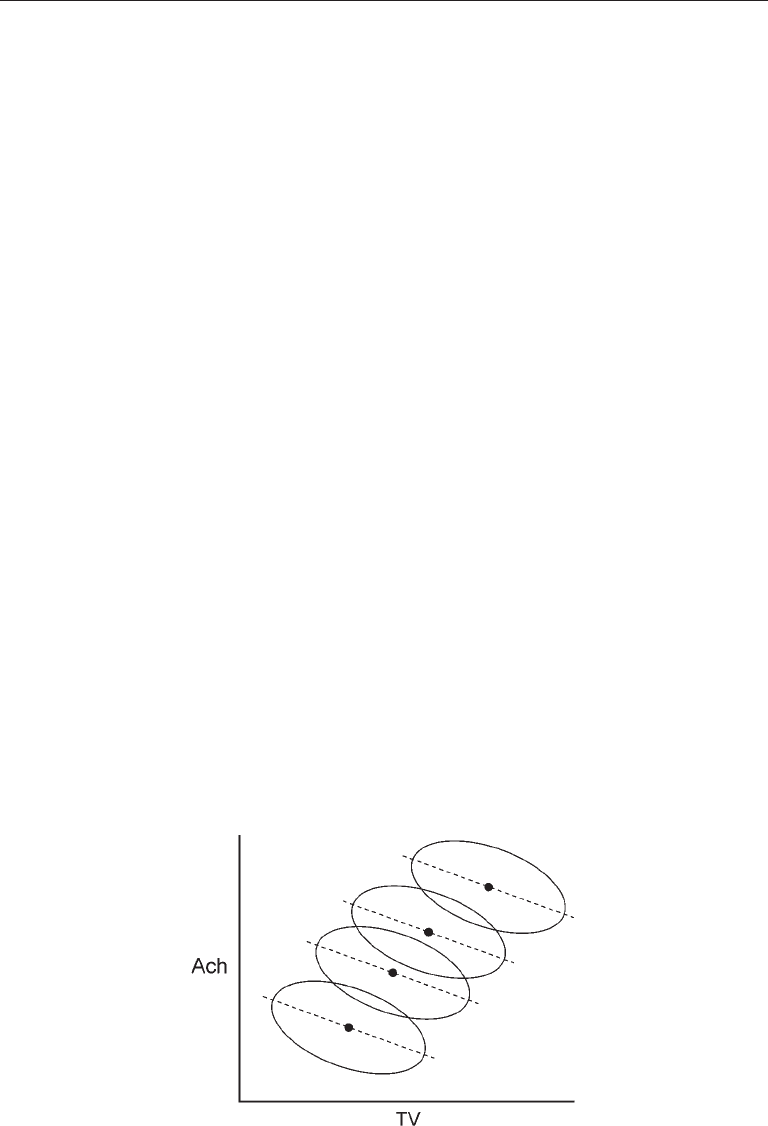
different levels are not always the same. Suppose that the amount of time spent watching

television (TV) and school achievement (Ach) are measured among students enrolled

in four different schools. Hypothetical scatterplots for these schools are presented in

Figure 12.6. Within each school, the association between TV and Ach is negative. That

346 ADVANCED TECHNIQuES, AVOIDING MISTAKES

is, more time spent watching television predicts lower achievement. From the perspec-

tive of traditional SEM, the same within-group covariance structure holds across the

schools.

But another aspect of the relation between TV and Ach in Figure 12.6 is apparent

from a between-group perspective: There is a positive association between the average

number of hours of television watched and the average achievement across the schools.

This positive covariance is apparent if you draw a line in the ﬁgure that connects the

four points that represent the group means (centroids) on both variables. The fact that

the within versus between relations of TV to Ach are of different signs in this example

is not contradictory. This is because the between association is estimated using group

statistics (school means), but the within association is estimated using scores from indi-

vidual students within the schools.

In Figure 12.6, the slopes of the within-school regression lines are identical. In a

two-level data set with a more realistic number of schools, such as 100 or so, it is more

likely that (1) both the slopes and the intercepts of the within regression lines will vary

across schools. Furthermore, (2) part of this variability over schools may be explained

by a contextual variable, such as school size. For example, the relation TV and Ach could

be stronger in smaller schools but closer to zero in larger schools. It can also happen that

(3) variability in slopes is related to variability in intercepts over schools. For example, a

weaker versus stronger association between Ach and TV (slopes) may predict lower ver-

sus higher mean scores on both variables (intercepts). That is, the covariance between

intercepts and slopes may not be zero.

All of the effects just mentioned can be estimated in a random coefﬁcient regres-

sion, in which data from predictors at ≥ 2 levels can be simultaneously analyzed. In

standard multiple regression (MR), slopes and intercepts are conceptualized as ﬁxed

population parameters. In contrast, slopes and intercepts in random coefﬁcient regres-

sion can be speciﬁed as random effects that vary and covary across the population of

clusters. Random coefﬁcient regression does not estimate the slope and intercept in any

FIgure 12.6. Representation of within-school versus between-school variation in the relation

between television watching (TV) and scholastic achievement (Ach).

Interaction Effects and Multilevel SEM 347

particular sample cluster. Instead, it uses sample information to estimate the population

variances and covariance of the slopes and intercepts. When a predictor, such as a con-

textual variable, of the random slopes or intercepts is speciﬁed, the model analyzed is

referred to as a slopes-and-intercepts-as-outcomes model. This means that the slopes

and intercepts from regression analyses at the case level (level 1) become the outcome

variables in the level-2 analysis where contextual variables are the predictors. Depending

on theory, it is also possible to specify that slopes only are random (slopes-as-outcomes

model) or that intercepts only are random (intercepts-as-outcomes model). The com-

plexity of the analysis increases quickly in designs with multiple level-1 or level-2 pre-

dictors or for hierarchical data sets with ≥ 3 levels (e.g., students within school within

districts). This is probably why most applications of random coefﬁcient regression in the

literature concern just two levels.

The OLS method is not the typical estimation method in random coefﬁcient regres-

sion. If the cluster sizes are all equal (a balanced design), then it may be possible to use

full-information maximum likelihood (FIML) as the estimator. This requires that the

number of clusters is reasonably large, say, > 75 or so, and also that the total number

of cases across all clusters is large, too (Maas & Hox, 2005). In unbalanced designs, it

may be necessary to use an approximate ML estimator, one that is computationally less

intensive but accommodates unequal cluster sizes. An example is restricted maximum

likelihood (REML), which is available in the Linear Mixed Models procedure of SPSS

and in the MIXED procedure of SAS/STAT. Another widely used computer program for

multilevel regression is Hierarchical Linear and Nonlinear Modeling (HLM) 6 (Rauden-

bush, Bryk, & Cheong, 2008).

Using the computer tools for multilevel analyses just

mentioned is relatively straightforward. For example, analyses can be speciﬁed in the

Linear Mixed Models procedure of SPSS with just a few clicks of the mouse cursor in

graphical dialogs or by writing a few lines of syntax (see Bickel, 2007).

Some limitations of MLM are as follows (Bauer, 2003; Curran, 2003):

1. Scores on individual- or cluster-level predictors in MLM are from observed vari-

ables that are assumed to be perfectly reliable. This is because there is no direct way in

MLM to represent measurement error.

2. There is also no direct way in MLM to represent either predictors or outcomes

as latent variables (constructs) measured by multiple indicators. In other words, it is dif-

ﬁcult to specify a measurement model as part of a multilevel analysis.

3. Although there are methods to estimate indirect effects apart from direct effects

in MLM, they can be difﬁcult to apply in practice (see Krull & MacKinnon, 2001).

4. There are statistical tests of individual coefﬁcients or of variances–covariances

in MLM, but there is no single inferential test of the model as a whole. Instead, the rela-

tive predictive power of alternative multilevel models estimated in the same sample can

be evaluated (e.g., Bickel, 2007, chap. 3).

A free student version of HLM 6 for Microsoft Windows is available at www.ssicentral.com/hlm/student.

html

348 ADVANCED TECHNIQuES, AVOIDING MISTAKES

ConvergenCe oF seM and MlM

The relative weaknesses of MLM correspond to the strengths of SEM. To summarize, it

is straightforward in SEM to represent measurement error for either single or multiple

indicators through the speciﬁcation of a measurement model. Factors can be represented

as either predictors or outcomes in a structural model. The estimation of direct or indi-

rect effects in structural models is a routine part of SEM, and there are inferential tests

of whether the model is consistent with the covariance data. But “unadorned” SEM has

limited capabilities in areas where MLM is strong. For example, the analysis of a model

across multiple samples in SEM is a kind of restricted multilevel analysis that assumes

ﬁxed population parameters for each group. Except when analyzing a particular class of

latent growth model in a single-level analysis (Chapter 11), SEM does not directly take

account of clustering in complex samples.

Early attempts to include more capabilities of MLM in SEM analyses were based on

tricking SEM computer tools into analyzing two-level models (e.g., Duncan, Duncan,

Hops, & Alpert, 1997). The trick was to exploit the capability of the software to simul-

taneously estimate a structural equation model across two groups. However, in this

case the “groups” corresponded to two different models, a within (level-1) model and a

between (level-2) model, both estimated in the same complex sample. The data matrix

for the level-1 model is the pooled within-group covariance matrix based on variation

of individual scores around cluster means. For the level-2 model, the data matrix is the

between-group covariance matrix based on variation of cluster means around the grand

means. Because older versions of most SEM computer programs had no built-in capabili-

ties for analyzing data from complex samples, it was usually necessary to calculate these

two data matrices separately using an external program, such as SPSS. The two data

matrices are then submitted to the SEM computer program as external ﬁles or included

as part of the syntax (command) ﬁle.

Unfortunately, the syntax required to trick older versions of SEM computer tools into

analyzing even relatively simple two-level models is awkward and complicated. Stapleton

(2006, p. 361) gives an example of such syntax for getting an SEM computer program to

analyze a two-level regression model that corresponds to the situation depicted in Figure

12.6. Just as awkward is the use of standard SEM symbolism for model diagrams to repre-

sent a multilevel analysis. For example, the model presented in Figure 12.7(a) represents

the trick just mentioned in McArdle–McDonald RAM symbolism for SEM, the system

used for model diagrams in this book. Brieﬂy, the observed variables TV and Ach are

each speciﬁed as the single indicator of a within-school factor and a between-school fac-

tor. The scaling constants for the within factors equal 1, but for the between factors these

constants equal the square root of the cluster size n

. At each level (within, between) of

the model in Figure 12.7(a), the Ach factor is regressed on the TV factor. These speciﬁca-

tions tell the computer to derive separate estimates of the within- and between-group

regression coefﬁcients. If the data resembled the pattern depicted in Figure 12.6, the

within coefﬁcient would be negative but the between coefﬁcient would be positive.

Interaction Effects and Multilevel SEM 349

Bauer (2003) and Curran (2003) show that it is even more complicated to use

standard SEM computer syntax to specify a slopes-and-intercepts-as-outcomes model.

The model requires both a mean structure and an individual factor loading matrix

where loadings on a slope factor are the scores from all the cases within each cluster.

Not all SEM computer programs allow the speciﬁcation of individual factor loading

matrices, but one that does is Mx (Chapter 4). The programming becomes even more

complicated if there are missing data or the cluster sizes are not all equal. Indeed, the

task quickly “becomes a remarkably complex, tedious, and error-prone task” (Curran,

2003, p. 557)—that is, a data management nightmare. Representation of a slopes-and-

intercepts-as-outcomes analysis with standard SEM symbolism for model diagrams is

relatively complex, too.

FIgure 12.7. Representation of a two-level regression model using (a) standard SEM symbolism

for model diagrams and (b) compact symbolism associated with Mplus.

350 ADVANCED TECHNIQuES, AVOIDING MISTAKES

MultIlevel seM

Fortunately, more and more computer programs for SEM, including EQS, LISREL, and

Mplus, feature special syntax that makes it easier to specify and analyze multilevel

models in complex samples. This special syntax is more compact to use for multilevel

analysis than standard SEM computer programming languages. It also allows for the full

integration of SEM and MLM in a framework known as multilevel structural equation

modeling (ML-SEM) that combines the capabilities of both families of techniques.

Because working with standard SEM model diagrams is not the best way to rep-

resent a multilevel analysis, the researcher typically conducts an ML-SEM analysis by

specifying the model in syntax, not in a graphical editor. An example of special syntax

in Mplus for analyzing a hypothetical slopes-and-intercepts-as-outcomes model is listed

in Table 12.4. The raw data from a complex sample are contained in an external ﬁle,

and the four observed variables are Ach, TV, School (attended), and Size (total enroll-

ment). Next, the syntax in Table 12.4 speciﬁes that TV is the within or level-1 predictor,

the cluster variable is School, and the between or level-2 predictor is Size. Grand-mean

centering of the TV variable is speciﬁed—centering is routine in this type of multilevel

analysis (Bickel, 2007)—and the analysis type is designated as two-level with random

coefﬁcients. Syntax for the within model speciﬁes that slopes, labeled “s” in the table,

from within the regressions of Ach on TV are a random variable. Syntax for the between

model speciﬁes that the random slopes and intercepts are regressed on the school size

contextual variable and that the random terms covary. See Stapleton (2006) for addi-

tional examples.

In the Mplus manual, Muthén and Muthén (1998–2010) use a special compact sym-

bolism for diagrams of multilevel structural equation models. For example, look back

at Figure 12.7(a), which is the standard diagram for tricking an SEM computer program

into analyzing a two-level regression model. Presented in Figure 12.7(b) is the model

taBle 12.4. example of special Mplus syntax for a hypothetical slopes-and-

Intercepts-as-outcomes Model

TITLE: Two-level slopes-and-intercepts-as-outcomes model

Students within schools

DATA: FILE IS “school.dat”;

VARIABLE: NAMES ARE Ach TV School Size;

WITHIN = TV; BETWEEN = Size;

CLUSTER = School; CENTERING = GRANDMEAN (TV);

ANALYSIS: TYPE IS TWOLEVEL RANDOM;

MODEL:

%WITHIN%

s | Ach ON TV;

%BETWEEN%

Ach s ON Size;

Ach WITH s;

OUTPUT: SAMPSTAT;

Interaction Effects and Multilevel SEM 351

for the same analysis but represented as an Mplus-type model diagram. This diagram

makes it clear that the regression of Ach on TV is calculated at two different levels,

within and between. It is also simpler than the standard representation in Figure 12.7(a).

Residual variance is represented in Figure 12.7(b) by the lines with arrowheads oriented

at 45° angles and pointing to the endogenous variables. This representation for residual

variance is compact, but does not convey the fact that residual terms are ordinarily con-

ceptualized as exogenous variables in an SEM analysis.

Another example of an Mplus-type diagram for a multilevel analysis is presented in

Figure 12.8. This model corresponds to the slopes-and-intercepts-as-outcomes model

speciﬁed in the syntax of Table 12.4. Random intercepts are represented in the within

model of Figure 12.8 by the closed circle at the end of the path TV → Ach, and random

slopes are represented by the closed circle in the middle of the same path. The random

slopes are labeled “s” in the ﬁgure. Random slopes and intercepts are represented in the

between model as latent variables that are regressed on school size, and the disturbances

for the random terms are speciﬁed as correlated. A mean structure is implied in Figure

12.8 because intercepts are estimated, but mean structures are not explicitly depicted in

Mplus-style diagrams. Curran and Bauer (2007) describe an alternative compact sym-

bolism for diagrams of multilevel structural equation models in which mean structures

are explicitly represented.

Using an SEM computer program with special syntax for multilevel analysis makes

possible the basic types of ML-SEM summarized next:

1. Estimation of correct standard errors when ﬁtting a single model to data from

a complex sample. This estimation takes account of the design effect and accordingly

corrects standard errors and test statistics.

2. Analysis of one model at the within level but another model at the between level.

The between model could be identical to the within model (e.g., Figure 12.7(b)), but the

between model could also be a different model. For example, a set of indicators may have

FIgure 12.8. Representation in Mplus-type symbolism of the slopes-and-intercepts-as-

outcomes model corresponding to the syntax in Table 12.4.

352 ADVANCED TECHNIQuES, AVOIDING MISTAKES

a three-factor structure at the within level, but at the between level the same indicators

measure a single factor.

3. Analysis of a slopes-and-intercepts-as-outcomes model where random slopes

and intercepts at the within level could be from either observed or latent variables that

are predicted by either observed or latent variables at the between level. Structural mod-

els at either level can include indirect effects.

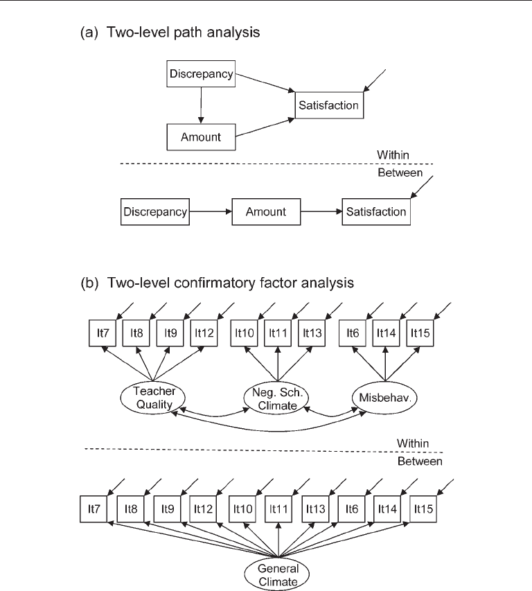
Two examples of ML-SEM analyses are described next. Wu (2008) administered

to 333 students a series of questionnaires about life satisfaction, what respondents say

they want (amount), and the gap between what they have and what they want (have–want

discrepancy) in 12 different areas (social support, ﬁnancial resources, etc.). Because rat-

ings across the 12 areas are repeated measures, Wu (2008) conceptualized these areas

as nested under individuals. That is, the within level concerns variation among areas

for each respondent, and the between level refers to differences across people that affect

their satisfaction ratings over all areas. In a multilevel path analysis (ML-PA), Wu

(2008) tested the hypothesis that have–want discrepancy and amount have direct or indi-

rect effects on life satisfaction. The ﬁnal path model retained in Wu’s (2008) analysis

is presented in Figure 12.9(a) using Mplus symbolism. At the within level, have–want

discrepancy has both direct and indirect effects on satisfaction. But at the between level,

effects of have–want discrepancy are entirely mediated by amount. Wu (2008) interpreted

these results as suggesting that life satisfaction involves an explicit have–want com-

parison, but whether its effect is entirely indirect through what people say they want

depends on the level of analysis, within-person versus between-person.

Kaplan (2000, pp. 48–53) describes a multilevel conﬁrmatory factor analysis

(ML-CFA) in a sample of over 10,000 high school students enrolled in about 1,000

different schools. The students completed a questionnaire about their perceptions of

teacher quality, negative school environment (e.g., students feel unsafe), and disruptive

behavior by students. In a single-level CFA ignoring clusters (schools), Kaplan (2000)

found that a three-factor model had reasonable ﬁt to item data. The ML-CFA model ana-

lyzed by Kaplan (2000) in the same sample is presented in Figure 12.9(b) using Mplus

symbolism where “It” designates “item.” The within model is basically identical to the

ﬁnal model retained in the single-level CFA. However, the model at the between level

is simpler in that all items load on a single factor. That is, variation in student ratings

within schools is differentiated along three dimensions, but one general climate fac-

tor explains between-school variation. For additional examples of ML-SEM analyses,

see Kaplan (2009, chap. 7), Mulaik (2009, chap. 12), and Rabe–Hesketh, Skrondal, and

Zheng (2007).

There are three basic steps in analyzing a multilevel structural equation model. The

ﬁrst step involves calculation of the unconditional intraclass correlation

. If

> .10,

the need for ML-SEM instead of single-level SEM is indicated. The next two steps parallel

those of the two-step estimation of SR models (Chapter 10), but in ML-SEM these steps

correspond to analysis of the within model only prior to simultaneous estimation of the

Interaction Effects and Multilevel SEM 353

within and between models. The goal is to distinguish speciﬁcation error in either level,

within versus between. Speciﬁcally, the within model is analyzed using the pooled-

within group covariances and means, which ignores the cluster variable. Although the

ﬁt of the within model may not be satisfactory due to the omission of between-group

effects, the basic parameter estimates should make sense. Finally, the between model is

speciﬁed, and then both models are simultaneously ﬁtted to the data. Stapleton (2006)

describes additional possible analytic steps.

FIgure 12.9. (a) Two-level path analysis model analyzed by Wu (2008). (b) Two-level

conﬁrmatory factor analysis model analyzed by Kaplan (2000).