Keyfitz N., Caswell H. Applied Mathematical Demography

Подождите немного. Документ загружается.

8.8. The Stable Equivalent 205

Table 8.9. Stable equivalents Q for United States females in 1960 and 1965, each

calculated with two diﬀerent matrices A (thousands)

Calculated with matrix A of

1960 1965

Age distribution:

1960 76,912 89,001

1965 85,478 98,645

Percent increase 11.14 10.84

Table 8.10. Stable equivalents Q for the United States and Mexico (thousands)

Calculated with matrix A of

United

States, Mexico,

1962 1962

Age distribution:

United States 82,933 63,395

Mexico 23,388 18,863

Ratio, Mexico to United States 0.282 0.272

1965 A. This way of making a comparison (applied between France and

Italy) is due to Vincent (1945), who noted the virtual invariance with re-

spect to the mortality and fertility patterns used. We are entitled to say

that the age distribution of women in the United States became about 11

percent more favorable to reproduction during the 5 years in question, and

the statement is true almost without regard to the fertility and mortality

patterns used in making this assessment.

As an example of a place comparison, Table 8.10 shows Q values for

Mexico and the United States, both for 1962. The Q for Mexico is 0.282

of that for the United States when the A of the latter is used; it is 0.272

when the A of the former is used. Jeﬀrey Evans has programmed place

comparisons among ﬁve countries which demonstrate the same invariance.

Section 12.3 below uses the stable equivalent to compare the eﬀect on age

distribution of eliminating cancer with that of eliminating heart disease.

8.8.4 A More General Stable Equivalent

Age is merely a special case of the stable equivalent. Any model that

possesses the ergodic property, that is, that tends asymptotically to a distri-

bution unaﬀected by the initial distribution, is equally capable of analysis

by the methods given above. In fact (8.8.3) remains unchanged; only now

the matrix A and the vector n(0) provide for the two sexes, regions, mar-

206 8. Reproductive Value from the Life Table

ried and single populations, and any other groups recognized in the model.

For details see Chapter 9 and some applications in Keyﬁtz (1969).

8.9 Reproductive Value as a Contribution to

Future Births

Section 8.1 appeals to intuition to make it appear likely that the eﬀect of

adding one girl or woman aged x to the population is to raise the number

of births t years hence, where t is large, in proportion to v(x)e

, v(x)being

deﬁned as

v(x)=



−ra

l(a)m(a) da

−rx

l(x)

This result can be derived from the Lotka equation of Section 7.5, but here

we examine a demonstration that is self contained, using the familiar device

of calculating the situation at time t from two successive moments near the

present. For purposes of this section v(x) will be deﬁned afresh, in terms

of the ultimate birth trajectory.

Suppose that a woman aged x at time zero contributes v(x)e

to the

births at subsequent time t,wherev(x)istobedeterminedandt is large.

This means that her disappearance would lower the ultimate birth trajec-

tory by v(x)e

. We assume that age-speciﬁc birth and death rates are ﬁxed,

so that her descendants will ultimately increase in geometric proportion and

be unaﬀected by other members of the population.

The woman aged x can, in the next short period of time and age, say ∆,

have a child, and whether or not she has a child can survive to the next

age, x + ∆. The chance of her having a child is m(x)∆, and the chance

of her surviving is l(x +∆)/l(x). By having a child she would contribute

v(0)e

r(t−∆)

to the births at time t, and by surviving she would convert

herself into a woman of reproductive value v(x + ∆) and so contribute

v(x +∆)e

r(t−∆)

. If the progression of childbearing and aging at the given

rates over the time ∆ is not to aﬀect the ultimate birth trajectory, we can

equate the two expressions for later births:

v(x)e



m(x)v(0)∆ +

l(x +∆)

l(x)

v(x +∆)



r(t−∆)

. (8.9.1)

If we multiply both sides of (8.9.1) by

∆

l(x)

v(0)

−rx

−rt

8.9. Reproductive Value as a Contribution to Future Births 207

we obtain

∆

l(x)

v(x)

v(0)

−rx

= m(x)l(x)e

−rx

−r∆

∆

l(x +∆)

v(x +∆)

v(0)

−r(x+∆)

(8.9.2)

Subtracting the rightmost term from both sides and letting ∆ → 0, we

have directly

−

l(x)

v(x)

v(0)

−rx

= m(x)l(x)e

−rx

and integrating gives

−rx

l(x)

v(x)

v(0)



−ra

l(a)m(a) da, (8.9.3)

so that, if v(0) is set equal to unity, v(x) again comes out as shown in

(8.1.1). No constant of integration is needed, since both sides are unity for

x = 0. Equation (8.9.3) establishes v(x) to within a multiplicative constant.

Let us ﬁnd the constant v(0) that corresponds to the ultimate eﬀect of

adding one female to the population.

If the initial age distribution is stable, we know that the population at

time t must be e

for each person initially present, and hence the births

at time t are be

. Equating the two values for time t,wehave



−rx

l(x)v(x) dx e

; (8.9.4)

since from (8.9.3) v(x) may be written as

v(0)

−rx

l(x)



−ra

l(a)m(a) da,

the be

−rx

l(x) within the integral of (8.9.4), as well as e

outside the

integral, cancels, and we obtain the following equation for v(0):

v(0)



−ra

l(a)m(a) da dx. (8.9.5)

The integral on the right-hand side is evaluated by integration by parts

and turns out to be κ, the mean age of childbearing in the stable population.

This proves that for the v(x) function of this section, v(0) = 1/κ, and that

the v(x) function of the main body of the chapter, deﬁned in (8.1.1), gives

the ultimate birth trajectory due to a woman aged x as e

v(x)/κ.

Reproductive Value from Matrix

Models

The concept of reproductive value is not limited to age-structured popu-

lations. It also applies to matrix population models for stage-structured

populations, where it appears as an eigenvector of the projection matrix.

9.1 Reproductive Value as an Eigenvector

We begin by returning to the projection equation

n(t +1)=An(t) n(0) = n

(9.1.1)

the solution of which (Section 7.1) can be written

n(t)=



, (9.1.2)

where λ

and w

are the eigenvalues and right eigenvectors of A and the

scalar constants c

are determined by the initial conditions n

;

c = W

−1

(9.1.3)

. (9.1.4)

The matrix W has the right eigenvectors w

as its columns; W

−1

has as

its rows the complex conjugate transposes of the left eigenvectors v

.Thus

= v

∗

(9.1.5)

with w

and v

scaled so that v

∗

=1.

9.1. Reproductive Value as an Eigenvector 209

If A is primitive, then

lim

t→∞

n(t)

= c

. (9.1.6)

The growth rate and stable population structure are independent of n

but the size of the population at any (large) time t depends on n

, through

the constant c

. From (9.1.5), c

is a weighted sum of the initial population,

with weights equal to the elements of v

Thus, if we take “the contribution of stage i to long-term population size”

as a reasonable measure of the “value of stage i,” the left eigenvector v

gives the relative reproductive values of the stages (Goodman 1968, Keyﬁtz

1968). We must insert the qualiﬁer “relative” because eigenvectors can be

scaled by any nonzero constant. The result c

= v

∗

holds when v

∗

1, but any other scaling can be accounted for by setting c

= v

∗

and eventual population size is still proportional to v

∗

. It is customary

to scale v

so that its ﬁrst entry is 1.

Regardless of the scaling imposed on v

, the total reproductive value

of a population, V (t)=v

∗

n(t), increases exponentially at the rate λ

regardless of the stage distribution:

V (t +1)=v

∗

n(t + 1) (9.1.7)

= v

∗

An(t) (9.1.8)

= λv

∗

n(t). (9.1.9)

9.1.1 The Eﬀect of Adding a Single Individual

Suppose that we add a single individual of stage j to the initial population

.Lete

be a vector with zeros everywhere except for a 1 in the jth entry.

If we drop the subscripts on λ

, w

and v

,wehave

lim

t→∞

+ e

)

= v

∗

+ e

) w (9.1.10)

= v

∗

w + v

w. (9.1.11)

The total population is v

∗

w + v

w, which diﬀers from (9.1.6) by

w. That is, adding a single individual in stage j increases asymptotic

population size by an amount proportional to the reproductive value of

stage j.

Reproductive Value and Extinction.

Any population is subject to stochastic ﬂuctuations because the vital rates

are probabilities applied to discrete individuals (demographic stochastic-

ity). These ﬂuctuations lead to a nonzero probability of extinction, even

when λ>1. This probability can be calculated for unstructured popula-

tions from the Galton–Watson branching process (see Section 16.4). The

corresponding probability for structured population is calculated from the

210 9. Reproductive Value from Matrix Models

multi-type branching process (Pollard 1973, MPM Chapter 15). In several

empirical examples (MPM Section 15.4.5), it has been shown that the prob-

ability of non-extinction of a population descended from a single founder

is directly proportional to the reproductive value of that founder. This

suggests, though it does not prove, that the reproductive value of an in-

dividual inﬂuences not only long-term population size but also short-term

risk of extinction.

9.1.2 Age-Speciﬁc Reproductive Value

We can write down the reproductive value for the age-classiﬁed case directly

from the equations deﬁning the eigenvector:

A = λv

where we have dropped the subscript, and are assuming that v is real.

Suppose there are four age classes, as in Figure 3.9a, and set v

=1.Then

1 v

⎛

⎜

⎝

000

0 P

00P

⎞

⎟

⎠

= λ

1 v

(9.1.12)

or, writing each equation out

+ v

= λ (9.1.13)

+ v

= λv

(9.1.14)

+ v

= λv

(9.1.15)

= λv

. (9.1.16)

From the last equation

= F

−1

. (9.1.17)

Substituting this into the next-to-last equation gives

= F

−1

+ P

−2

(9.1.18)

and then

= F

−1

+ P

−2

+ P

−3

. (9.1.19)

Finally, substituting this into the ﬁrst equation gives

1=F

−1

+ P

−2

+ P

−3

+ P

−4

(9.1.20)

which is the characteristic equation (see Example 7.1). In general the age-

speciﬁc reproductive value is



j=i



j−1

h=i



i−j−1

, (9.1.21)

9.1. Reproductive Value as an Eigenvector 211

-1

2 3 4

-1

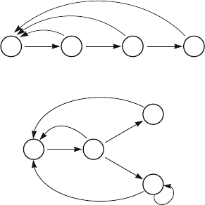
Figure 9.1. The transformed graphs for two life cycles. Above: an age-structured

model with four age classes. Below: a hypothetical life cycle in which individuals

of stage N

have two developmental choices, in one of which (N

) they reproduce

only once and in the other of which (N

) they survive with probability P

and

reproduce repeatedly.

which is the discrete version of Fisher’s formula (8.1.1).

9.1.3 Stage-Speciﬁc Reproductive Value and the Life Cycle

Graph

We can understand the correspondence of the left eigenvector and repro-

ductive value in stage-structured models by writing down the eigenvector

directly from the life cycle graph (Caswell 1982a; see Chapter 7 of MPM for

details). Begin by transforming the life cycle graph by replacing each coeﬃ-

cient a

with a

−1

. (This is known as the z-transform of the graph; in our

context, however, the variable usually denoted by z will be the eigenvalue

of A, so we denote it as λ.)

Figure 9.1 shows the transformation of the life cycle graph for the age-

classiﬁed model. Comparing this graph with (9.1.17)–(9.1.20), we see that

is the sum, over all pathways from N

to N

, of the product over each

pathway of the transformed life cycle graph coeﬃcients. There are, for

example, two pathways from N

to N

. The products of the transformed

coeﬃcients on these pathways are F

−1

and P

−2

; the sum of these is

in (9.1.18).

In other words, v

measures the expected future reproductive contribu-

tion from stage N

, discounted by the population growth rate and the time

212 9. Reproductive Value from Matrix Models

required for the contribution; e.g.,

= F

−1

2 34 5

1 step

+ P

−2

2 34 5

2steps

+ P

−3

2 34 5

3steps

. (9.1.22)

This algorithm gives the left eigenvector for a wide class of life cycles.

∗

In the (imaginary) stage-classiﬁed life cycle of Figure 9.1b, an individual

in N

may proceed to a stage (N

) in which it only reproduces once or to

a stage (N

) in which it survives indeﬁnitely with a probability P

.The

resulting reproductive value vector, obtained by summing contributions

from each stage back to the ﬁrst, is

= 1 (9.1.23)

= F

−1

+ P

−2

1 − P

−1

(9.1.24)

= F

−1

(9.1.25)

−1

1 − P

−1

. (9.1.26)

Each of these values is clearly a measure of future contribution to births,

discounted by the population growth rate.

†

Residual Reproductive Value.

Equation (8.9.1) decomposed reproductive value at age x into two compo-

nents, one from reproduction at age x and the other from survival to,

and reproduction at, later ages. These components were called current

reproduction and residual reproductive value by Williams (1966). In the

age-classiﬁed case (9.1.12), e.g.,

= F

−1

+ P

−1

, (9.1.27)

where the ﬁrst term is current reproduction and the second is residual

reproductive value. In the stage-classiﬁed example, an individual in N

has

two possible fates, so

= F

λ−1+P

−1

+ R

−1

. (9.1.28)

The ﬁrst term is current reproduction and the second two terms together

constitute residual reproductive value.

∗

Including any life cycle in which all loops other than self-loops pass through N

If there are more complicated loop structures, additional terms are required (Caswell

1982a, MPM Chapter 7).

†

The terms

1 − P

=1+P

−1

+ P

−2

+ ...

created by the self-loop on N

reﬂect the probability that the individual will remain in

for 1, 2,... time steps.

9.2. The Stable Equivalent Population 213

9.2 The Stable Equivalent Population

The stable equivalent population of Section 8.8 applies to any classiﬁcation

of individuals (Keyﬁtz 1969). An initial population n

with an arbitrary

stage distribution will asymptotically produce an exponentially growing

population of the same size as an initial population of size Q with the

stable stage distribution.

To calculate Q, we scale w so that w =1,andv so that v

∗

w =1.

The population starting at n

will eventually grow as

lim

t→∞

n(t)

= v

∗

w (9.2.1)

while that starting from n(0) = Qw will grow as

lim

t→∞

n(t)

= Q (v

∗

w) w. (9.2.2)

Equating the two gives

Q = v

∗

. (9.2.3)

That is, the stable equivalent is just the total reproductive value of the

initial population, when scaled so that w = 1 and v

∗

w =1.

We note in passing that the models considered here and in Chapter 8

describe constant environments. Tuljapurkar and Lee (1997) have extended

the stable equivalent concept to models in which the vital rates ﬂuctuate

stochastically in time.

Example 9.1 Stable equivalent for the killer whale

Killer whales (Orcinus orca) live in stable social groups called pods.

A life cycle is shown in Figure 3.10, and a set of vital rates estimated

from an intensively studied population of 18 pods in coastal waters

of Washington and British Columbia is shown in Example 11.1. The

right and left eigenvectors, appropriately scaled, are

w =

⎛

⎜

⎝

0.037

0.316

0.323

0.324

⎞

⎟

⎠

v =

⎛

⎜

⎝

1.142

1.198

1.794

⎞

⎟

⎠

. (9.2.4)

Each pod has its own observed structure, and Table 9.1 compares the

stable equivalent and the observed population of each. In contrast to

the comparison of the stable and observed population sizes of 12

countries in Table 8.8, which were within a few percent of each other,

among killer whale pods the stable equivalent ranges from 22 percent

smaller to 71 percent larger than the observed population. When Q<

N, the population is biased toward individuals of low reproductive

value, and vice versa.

214 9. Reproductive Value from Matrix Models

Table 9.1. The observed female population (N = n) and the stable equivalent

population Q for each of 18 pods of resident killer whales (Orcinus orca)in

Washington and British Columbia.

12.93 10.59 0.82

10.30 8.05 0.78

26.23 28.10 1.07

5.77 5.77 1.00

4.20 6.33 1.51

7.73 9.48 1.23

1.23 2.11 1.71

5.10 4.74 0.93

5.63 6.69 1.19

11.53 12.27 1.06

5.13 7.33 1.43

3.07 4.82 1.57

2.50 3.78 1.51

2.30 1.99 0.87

6.37 9.12 1.43

6.13 9.00 1.47

2.93 4.22 1.44

8.47 11.71 1.38

The inﬂuence of n

on eventual population size (and probability of

extinction) is of more than academic interest in conservation biology. In-

vasions of introduced animals and plants create huge environmental and

economic problems around the world. Studies of the determinants of in-

vasion success of birds and mammals in New Zealand (which, because of

its isolation, has been particularly vulnerable to invasions) have shown a

correlation between the size of the introduced population and the success

of the invasion (Veltman et al. 1996, Forsyth and Duncan 2001). The stable

equivalent of the introduced population might be even more relevant.

The eﬀect of initial population also arises in attempts to reintroduce

threatened species to areas from which they have been exterminated. This

is an increasingly frequent task; at this writing, 132 such projects involving

63 species are underway in New Zealand alone. Many of these involve intro-

ductions of individuals to oﬀshore islands from which introduced predators

have been eliminated. All else being equal, it might be useful to try to

maximize the stable equivalent population size in such introductions.