Keyfitz N., Caswell H. Applied Mathematical Demography

Подождите немного. Документ загружается.

7.4. Computation of Eigenvalues and Eigenvectors 175

reproduction by these individuals generates an increase in population

size once the vital rates change to stationarity.

Dividing fertilities by R

is not the only way to achieve a set of stationary

vital rates. Changes in survival or transition probabilities could also be

used, and might have diﬀerent consequences for momentum. It is unlikely

that the vital rates could be changed instantaneously to replacement level.

Li and Tuljapurkar (1997) have considered the more general problem of an

arbitrary change in the vital rates, over some speciﬁed period of time, from

the old to the new stationary rates.

7.4 Computation of Eigenvalues and Eigenvectors

The numerical calculation of eigenvalues and eigenvectors is not an easy

problem. In their compilation of numerical recipes, Press et al. (1986) call

it “one of the few subjects covered in this book for which we do not recom-

mend that you avoid canned routines.” See Wilkinson (1965) and Wilkinson

and Renisch (1971) for the details if you really want to try it yourself.

Fortunately, there are now a number of computer packages available for

matrix calculations. By far the best is Matlab.

‡

It is available for most

platforms and operating systems, permits both interactive calculations and

the writing of complex programs, contains powerful graphics capabilities,

and is widely used in the mathematics, physics, and engineering commu-

nities. The availability of this software and the power of microcomputers

have revolutionized demographic calculations involving matrices.

7.4.1 The Power Method

The dominant eigenvalue of A, and the corresponding eigenvectors, can be

easily computed by the power method. If A is primitive,

lim

t→∞

= w

. (7.4.1)

For large t,thecolumnsofA

are eventually all proportional to w

;the

rows are all proportional to v

. The eigenvalue λ

can be calculated as the

ratio of any entry of A

t+1

to the corresponding entry of A

The entries of A

may overﬂow or underﬂow the computer for large t.

This can be avoided by rescaling A

at each time step (e.g., divide A

‡

The MathWorks, Inc., 3 Apple Hill Drive, Natick MA, 01760, U.S.A.;

http://www.mathworks.com.

For example, as of this writing, computing all the eigenvalues and eigenvectors of a

100×100 matrix in Matlab takes less than 0.1 seconds on an ordinary laptop computer.

A 500 × 500 matrix takes only 6.5 seconds.

176 7. Birth and Population Increase from Matrix Population Models

its maximum entry, so that all values remain between 0 and 1). Wilkinson

(1965, Chapter 9) discusses the extension of the power method to ﬁnd the

subdominant eigenvalues and their eigenvectors.

7.5 Mathematical Formulations of the Basic

Equation of Population

So far, this book has dealt with what in retrospect can be seen as special

cases of a general analysis. Chapter 2 treated the pure death process of the

life table, in which births, if considered at all, were just equal to deaths.

Chapter 5 used the life table along with an arbitrary rate of increase r to

constitute a stable age distribution. Chapters 6 and 7 ascertained the same

r from equations incorporating age-speciﬁc birth rates as well as the life

table.

The general analysis of which all these are parts relates the entire popu-

lation of each generation or period to the preceding. This can be done in the

form of an integral equation, a matrix multiplication, a diﬀerence equation,

and a partial diﬀerential equation.

Because all these methods distinguish

individuals on the basis of some i-state variables, they are referred to in gen-

eral as structured population models; for a discussion with many ecological

examples see the chapters in Tuljapurkar and Caswell (1997).

These mathematical forms look very diﬀerent from one another, though

they are ultimately equivalent. The purpose of presenting them is not to

exhibit the mathematical virtuosity of their several authors, but to take

advantage of the fact that some applications are easier with one approach,

others with another. This book is not the place to treat the mathematics

in detail; that has been done elsewhere (Coale 1972, Pollard 1973, Keyﬁtz

1968, Rhodes 1940, Tuljapurkar and Caswell 1997). Here the several ap-

proaches will be presented, and some observations made on their relation

to one another and to the applications that are the subject of this book.

7.5.1 The Lotka Integral Equation

Historically the earliest formulation was in terms of an integral equation

solved by Sharpe and Lotka (1911), whose unknown is the trajectory of

births and which, under the name of the renewal equation, has become

famous in many other contexts. Births B(t)attimet are the outcome of

the births a years earlier, where a ranges from about 15 to about 50, say

from α to β in general. Newborns of a years earlier, numbering B(t − a),

There is also a large literature using delay-diﬀerential equations for the same purpose

(Nisbet 1997, Gurney and Nisbet 1998) and a small but growing literature on systems

of integrodiﬀerence equations (Neubert and Caswell 2000, Easterling et al. 2000).

7.5. Mathematical Formulations 177

have a probability l(a) of surviving to time t: those that do survive have

a probability m(a) da of themselves giving birth in the time interval a to

a + da; the total of these over ages α to β is



B(t −a)l(a)m(a) da,which

ultimately must equal current births B(t). But any such system has to have

an initial condition to start it oﬀ; in the Lotka equation the initial condition

is G(t), the number of births due to the women already born at the start

of the process. The function G(t) is zero for t  β, when all the females

alive at t = 0 have passed beyond childbearing. Entering the known G(t)

and l(a)m(a) in the Lotka integral equation,

B(t)=



B(t − a)l(a)m(a) da + G(t), (7.5.1)

determines the trajectory B(t).

The method used by Lotka to solve (7.5.1) for B(t) was ﬁrst to deal with

the homogeneous form, in which G(t) is disregarded, and to try B(t)=e

Entering this value for B(t) and corresponding B(t−a)=e

r(t−a)

in (7.5.1)

without G(t) gives the characteristic equation (6.1.2), which has for the

general net maternity function l(a)m(a) an inﬁnite number of roots. This

is a more satisfactory way of deriving (6.1.2) than was used above. The

left-hand side of (6.1.2), say ψ(r), is large for negative r and diminishes

toward zero as r becomes large and positive; we saw that only one of the

roots can be real. Suppose that the roots in order of magnitude of their

real parts are r

, r

,.... The complex roots, such as the pair r

, r

must be pairs of complex conjugates, say x + iy, x −iy,wherex and y are

real; if they are not conjugates, they could not be assembled into the real

equation (6.1.2).

The homogeneous form [i.e., omitting G(t) from (7.5.1)] is linear, and

hence if e

is a solution so is Q

,whereQ

is an arbitrary constant. If

a number of such terms are solutions, so is their sum. These considerations

provide the general solution to the homogeneous form

B(t)=Q

+ Q

+ ···, (7.5.2)

where the r’s are the roots of (6.1.2) and the Q’s are arbitrary constants.

The solution to the nonhomogeneous form (7.5.1) containing G(t)isob-

tained by selecting values of Q that accord with the births G(t)tothe

initial population. Lotka showed that these are



−r

G(t) dt



−r

l(a)m(a) da

s =1, 2,.... (7.5.3)

The constant Q

attached to the real term will be important in Chapter 6,

where we seek the eﬀect on the trajectory of adding one person aged x.

178 7. Birth and Population Increase from Matrix Population Models

A less awkward way to solve (7.5.1) (Feller 1941, Keyﬁtz 1968, p. 128) is

by taking the Laplace transform of the members. That of B(t), for example,

∗

(r)=



∞

−rt

B(t) dt

and similarly for G(t)andl(a)m(a)=φ(a), say. The integral on the right of

(7.5.1) is a convolution, that is to say, the sum of the arguments of the two

functions B(t − a)andl(a)m(a)=φ(a) in the integrand does not involve

a; the transform of a convolution is the product of the transforms of the

two functions. The equation in the transforms (distinguished by asterisks)

is thus

∗

(r)=G

∗

(r)+B

∗

(r)φ

∗

(r),

and is readily solved for the transform B

∗

(r) of the unknown function B(t):

∗

(r)=

∗

(r)

1 − φ

∗

(r)

To invert the right-hand side, expand in partial fractions, using the factors

of 1 − φ

∗

(r), obtained from the roots r

, r

,...,ofφ

∗

(r)=1,whichisthe

same as (6.1.2). Call the expansion of B

∗

(r)

∗

(r)=

r − r

+ ···.

The Laplace transform of e



∞

−rt

dt =

r − r

as appears from integration, so the inverse transform of 1/(r − r

)ise

Using this fact permits writing the solution in the form of (7.5.2), and the

coeﬃcients Q

are the same as before, that is, (7.5.3). Specializing (7.5.3)

to s = 1 gives the constant Q

for the ﬁrst term of the solution as



−rt

G(t) dt

, (7.5.4)

where again κ is the mean age of childbearing in the stable population. The

roots r

, r

,...,all have real parts less than r

, so the terms involving them

become less important with time, and the birth curve B(t) asymptotically

approaches Q

. This statement holds under general conditions on φ(a)

analogous to those of Section 1.10.

What the solution (7.5.2) amounts to is a real term that is an expo-

nential, plus waves around this exponential, of which the demographically

interesting one corresponds to the pair of complex roots of largest absolute

7.5. Mathematical Formulations 179

value, has the wavelength of the generation, and accounts for the echo ef-

fect: other things being constant, a baby boom in one generation is followed

by a secondary baby boom in the next generation.

7.5.2 The Leslie Matrix

The age-classiﬁed Leslie matrix, from which the stage-classiﬁed models in

this chapter evolved, can be traced back to Whelpton’s (1936) presentation

of what he called the components method of population projection, in which

an age distribution in 5-year age groups is “survived” along cohort lines,

and births less early childhood deaths are added in each cycle of projection.

The method was also used by Cannan (1895) and Bowley (1924) after him.

The dominant eigenvalue of a Leslie matrix, using a k-year projection

interval, corresponds to e

of the Lotka formulation with time measured

in years. With ﬁnite age groups, in the usual ﬁnite approximation, the pop-

ulation grows somewhat faster on the Leslie than on the Lotka projection;

for instance, over a 5-year period, using Mexican data for 1966, λ

was

1.1899 whereas e

was 1.1891. For a low-increase country like the United

States the diﬀerence does not show by the fourth decimal place, and it

vanishes altogether when the projection interval is made small. In fact, as

the interval becomes small, the two models become identical (Keyﬁtz 1968,

Chapter 8).

7.5.3 The Diﬀerence Equation

A third way of looking at the population trajectory, developed like the

matrix during the 1930s and 1940s, by Thompson (1931), Dobbernack and

Tietz (1940, p. 239), Lotka (1948, p. 192), and Cole (1954, p. 112), is in

terms of a diﬀerence equation. A secondary treatment is found in Keyﬁtz

(1968, p. 130). Although the approach is now mainly of historical interest,

it is still occasionally used (e.g., Croxall et al. 1990).

Consider one girl baby together with the series expected to be generated

byherat5-yearintervals,sayu

, u

,..., where u

= 1. The simplest

way to describe the model is to bunch the person-years lived into points at

5-year intervals. The u

will at ﬁrst decrease, corresponding to the probabil-

ity that the girl will die during the time before she begins to bear children;

then they will start to increase, and they will increase further with the

approach to u

just 40 years later, when her children start to bear. The

series generated by the girl now alive includes the probability that she will

live for 15 years and then have a child, say a probability of f

, that she

will live 20 years and then have a child, f

, and so on. After n periods of

5 years the girl’s descendants (including herself if still alive) are u

.The

must be equal to the chance of her living that long and having a child

then, f

, plus the chance of her having lived n −1 periods and having a

180 7. Birth and Population Increase from Matrix Population Models

child that would now have given rise to u

,andsoon.Insum,

= f

+ f

n−1

+ f

n−2

+ ··· (7.5.5)

for all n. In this series the f are known quantities corresponding to the

l(a)m(a) of the Lotka form, or to the P

of the matrix; the u seriesisthe

unknown function corresponding to B(t − a).

Just as the integral equation was solved by the Laplace transform, so

(7.5.5) is solved by generating functions. Multiply (7.5.5) for u

by s

,add

all such equations from n =0ton = ∞, and then express the result in

terms of

U(s)=u

+ u

s + u

+ ···,

F (s)=f

+ f

s + f

+ ···,

so that the set of equations 7.5.5 amounts to

U(s)=1+U (s)F (s),

which is readily solved to give

U(s)=

1 − F (s)

. (7.5.6)

Dividing out the right-hand side would only generate again the series

with which we started. But ﬁrst ﬁnding the roots of 1 −F (s) = 0, a further

form of the characteristic equation, using the roots to break down the right-

hand side of (7.5.6) into partial fractions of the type d

/(s − s

), and then

expanding each of the partial fractions, we get a series in powers of s that

corresponds to (7.5.2) in the Lotka solution.

The descriptions read as though the Lotka model is backward look-

ing, since it ﬁnds the relation between the present generation and the

preceding one, whereas the Leslie model and the set of diﬀerence equa-

tions are forward looking, portraying the continuance of present rates into

the future. These diﬀerences of direction are superﬁcial, however, and the

mathematical outcomes are essentially identical.

7.5.4 The McKendrick–von Foerster Equations

A fourth approach, due to McKendrick (1926, Kermack and McKendrick

1927) and von Foerster (1959), uses partial diﬀerential equations, with both

age and time continuous variables. It is most easily visualized in terms of the

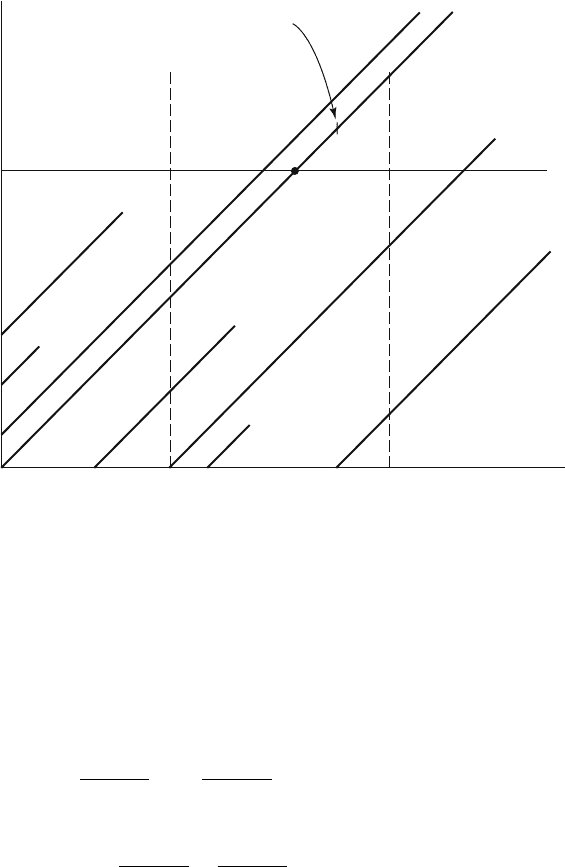
Lexis diagram (Figure 2.1), redrawn in the present context as Figure 7.7.

If P(a, t) is the population (say of females) at age a and time t, the female

population of age a+∆a at time t+∆t is P (a+∆a, t+∆t). If ∆a =∆t the

latter includes the same individuals as were counted in P (a, t), only subject

to deductions for mortality (as well as for emigration if one wishes, but

the present section excludes migration). The equation of change involving

7.5. Mathematical Formulations 181

(a, t)

(a + ∆a, t + ∆ t)

Age

Time

P(0, t)

P(a, 0)

␣␤

Reproductive ages

Figure 7.7. Lexis diagram showing boundary distributions P (a, 0) along age axis

given at the outset, and P (0,t) along time axis generated by (7.5.8) and (7.5.9);

(7.5.8) ﬁlls out the interior of the quadrant.

mortality µ(a), a function of age but not of time, is

P (a +∆a, t +∆t)=P (a, t) − µ(a)P (a, t)∆t. (7.5.7)

Expanding P (a +∆a, t +∆t) by Taylor’s theorem for two independent

variables and canceling P (a, t) from both sides leaves

∂P(a, t)

∂t

∆t +

∂P(a, t)

∂a

∆a = −µ(a)P (a, t)∆t.

Dividing by ∆a, which is equal to ∆t,wehave

∂P(a, t)

∂t

∂P(a, t)

∂a

= −µ(a)P (a, t). (7.5.8)

This is the McKendrick–von Foerster partial diﬀerential equation for one

sex, for all values of 0 <a<ω,whereω is the oldest age to which anyone

lives.

Births enter as a boundary condition at age zero:

P (0,t)=



P (a, t)m(a) da, (7.5.9)

182 7. Birth and Population Increase from Matrix Population Models

where α is the youngest age of childbearing and β the oldest, and m(a)is

the age-speciﬁc birth rate, supposed to be invariant with respect to time.

This derivation assumes that a represents age, but these models have

been extended to classiﬁcation by size or physiological condition by

Sinko and Streifer (1967, 1969), Oster (1976), and van Sickle (1977a,b).

For density-dependent versions see Gurtin and MacCamy (1974), Oster

and Takahashi (1974), and Oster (1976). The monograph of Metz and

Diekmann (1986) provides a complete but mathematically challenging

treatment; de Roos (1997) provides the best introduction for beginners.

In the general model, let g(a, t) be the “growth rate”, that is, the rate

at which individuals increase in whatever characteristic a represents. Then

(7.5.8) becomes

∂P(a, t)

∂t

∂g(a, t)P (a, t)

∂a

= −µ(a)P (a, t). (7.5.10)

For the special age-classiﬁed case, g(a)=1.

7.5.5 A Common Structure

The common structure of the four presentations may not stand out

conspicuously, but each has the following.

1. An initial age distribution.

2. Provision for mortality; in the ﬁrst three methods this is the sur-

vival probability l(x)orL

of the life table, while in the von Foerster

method it is the age-speciﬁc death rate µ(a); if age and time move for-

ward together we have a cohort, and the partial diﬀerential equation

whose solution is

l(x)=exp



−



µ(a) da



3. Provision for reproduction, presented as the ﬁrst row of the matrix

A, and as the boundary condition (7.5.9) in the partial diﬀerential

equation.

4. A characteristic equation, whose real or positive root is the intrinsic

rate or its exponential, obtained from the birth boundary condition

in the partial diﬀerential equation.

5. Right eigenvectors, of which the positive one is the stable age distri-

bution.

6. Left eigenvectors, of which the positive one contains the reproductive

values of the several ages or stages (Chapters 8 and 9).

In principle any property of the deterministic population process under

a ﬁxed regime is obtainable from any of the four forms, and numerical

diﬀerences disappear if the interval of time and age is small enough.

Reproductive Value from the Life

Table

When a woman of reproductive age is sterilized and so has no further chil-

dren, the community’s subsequent births are reduced. When a woman dies

or otherwise leaves the community, all subsequent times are again aﬀected.

Our formal argument need make no distinction between emigration and

death, between leaving the country under study for life and leaving this

world altogether. A single theory answers questions about the numerical

eﬀect of sterilization, of mortality, and of emigration, all supposed to be

taking place at a particular age x. By means of the theory we will be able

to compare the demographic results of eradicating a disease that aﬀects

the death rate at young ages, say malaria, as against another that aﬀects

the death rate at older ages, say heart disease.

A seemingly diﬀerent question is what would happen to a rapidly increas-

ing population if its couples reduced their childbearing to bare replacement

immediately. The period net reproduction rate R

, the number of girl chil-

dren expected to be born to a girl child just born, would equal 1 from then

on, and ultimately the population would be stationary. But the history of

high fertility has built up an age distribution favorable to childbearing, and

the ultimate stationary total will be much higher than the total at the time

when the birth rate dropped to bare replacement. The amount by which

it will be higher is calculable, and by the same function—reproductive

value—that is used for problems of migration and changed mortality.

184 8. Reproductive Value from the Life Table

8.1 Concept of Reproductive Value

Without having these particular problems in mind, Fisher (1930, p. 27)

developed a fanciful image of population dynamics that turns out to provide

solutions to them. He regarded the birth of a child as the lending to him of

a life, and the birth of that child’s oﬀspring as the subsequent repayment

of the debt. Apply this to the female part of the population, in which the

chance of a girl living to age a is l(a), and the chance of her having a girl

between ages a and a + da is m(a) da, so that the expected number of

children in the small interval of age speciﬁed is l(a)m(a) da. This quantity

added through the whole of life is what was deﬁned as the net reproduction

rate R

in Section 6.1:



l(a)m(a) da,

where α is the youngest age of childbearing and β the oldest. The quantity

is the expected number of girl children by which a girl child will be

replaced; for the population it is the ratio of the number in one generation

to the number in the preceding generation, according to the given l(a)and

m(a) (see Chapter 9 for the generalization to stage-classiﬁed models).

Fisher’s image discounts the future, at a rate of interest equal to the

intrinsic rate r of Section 6.1. The value of 1 dollar, or one child, discounted

back through a years at annual rate r compounded momently is e

−ra

;

therefore the value of l(a)m(a) da children is e

−ra

l(a)m(a) da,asinthe

ﬁnancial calculations of Section 2.5. The present value of the repayment

of the debt is the integral of this last quantity through the ages to the

end of reproduction. Thus the debt that the girl incurs at birth is 1, and

the discounted repayment is the integral



−ra

l(a)m(a) da. If loan and

discounted repayment are to be equal, we must have



−ra

l(a)m(a) da,

and this is the same as the characteristic equation (Lotka 1939, p. 65, and

(6.1.2)), from which the r implied by a net maternity function l(a)m(a)is

calculated. The equation can now be seen in a new light: the equating of

loan and discounted repayment is what determines r, r being interpretable

either as the rate of interest on a loan or as Lotka’s intrinsic rate of natural

increase.

The loan-and-repayment interpretation of the characteristic equation

suggests calculating how much of the debt is outstanding by the time the

girl has reached age x<β. This is the same as the expected number of

subsequent children discounted back to age x. Her expected births in the

interval a to a + da, a>x,are[l(a)/l(x)]m(a); and if these births are