Keyfitz N., Caswell H. Applied Mathematical Demography
Подождите немного. Документ загружается.


6.6. Moments of Dying and Living Populations 145
The exponential of the cumulant-generating function of the ages of the
dying is
exp[ψ(r)] =
ω
0
e
−rx
l(x)µ(x) dx = −
ω
0
e
−rx
dl(x),
and on integration by parts we have
−
ω
0
e
−rx
dl(x)=−e
−rx
l(x)|
ω
0
− r
ω
0
e
−rx
l(x) dx
=1− r
ω
0
e
−rx
l(x) dx.
But the integral here is
ω
0
l(x) dx times the exponential of the cumulant-
generating function of the living. Hence there follows the identity
exp[ψ(r)]=1− r
o
e
0
exp[ψ
L
(r)], (6.6.2)
where ψ
L
(r)=log[
ω
0
e
−rx
l(x) dx/
ω
0
l(x) dx], referring to the living, is
distinguished from ψ(r)=log[
ω
0
e
−rx
l(x)µ(x) dx], referring to the dying.
Note that
ω
0
l(x)µ(x) dx = 1; therefore we do not need a denomina-
tor for ψ(r), generating the cumulants of the dying, but do require the
denominator
ω
0
l(x) dx =
o
e
0
for ψ
L
(r).
The basic result is (6.6.2); and, subject to conditions of convergence that
do not seem to give trouble in practice, expanding ψ(r)andψ
L
(r)within
it enables us to find one set of cumulants in terms of the other:
exp
−
o
e
0
r +
σ
2
r
2
2
−
κ
3
r
3
6
+ ···
=
1 − r
o
e
0
exp
−µ
L
r +
σ
2
L
r
2
2
−
κ
3L
r
3
6
+ ···
,
or on expanding the exponentials
1 −
o
e
0
r +(σ
2
+
o
2
e
0
)
r
2
2
−···=
1 − r
o
e
0
1 − µ
L
r +(σ
2
L
+ µ
2
L
)
r
2
2
−···
.
Equating powers of r,weget
o
e
0
=
o
e
0
σ
2
+
o
2
e
0
2
=
o
e
0
µ
L
κ
3
+3σ
2
o
e
0
+
o
3
e
0
6
=
o
e
0
(σ
2
L
+ µ
2
L
)
2
and so on.

146 6. Birth and Population Increase from the Life Table
Thus σ
2
=2
o
e
0
µ
L
−
o
2
e
0
, identically, and we have without approximation
the variance in the age of dying in terms of the mean age of the living and
o
e
0
, all for the life table population. For example, in the case of Colombian
females, 1964, where
o
e
0
=61.563 and µ
L
=37.360, the variance in age at
death is
σ
2
= 2(61.563)(37.360) − (61.563)
2
= 810.0.
Thus the four cumulants of ages in a stationary population given for some
200 populations in Keyfitz and Flieger (1968) provide five cumulants of
ages of the dying for those same populations.
6.6.1 Expectation of Life as a Function of Crude Birth and
Death Rates
If we know only the crude death rate of a population we can say little about
its expectation of life; a crude death rate of 10 can apply to a country with
a life expectation as high as 75 years or as low as 60 years, in the former
case with a rate of increase of 0.005 and in the latter of 0.030. If we are
also told the crude birth rate or the rate of natural increase, we can narrow
this range considerably, as McCann (1973) has shown.
We know that d, the crude death rate in the stable population, is
d =
ω
0
be
−ra
l(a)µ(a) da,
so that, dividing by b and noting that the right-hand side is the exponential
of the cumulant-generating function of the distribution of deaths by age
expressed in terms of −r,wehave
d
b
=
ω
0
e
−ra
l(a)µ(a) da,
or log d − log b = ψ(r), and this is the same as
log b − log d = r
o
e
0
−
r
2
σ
2
2
+
r
3
κ
3
6
−···,
since in the stationary population the mean age of dying is the expectation
of life
o
e
0
. Solving for
o
e
0
gives
o
e
0
=
log b − log d
b − d
+ r
σ
2
2
−
rκ
3
6
+
r
2
κ
4
24
−···
, (6.6.3)
where r = b − d. Now the expression in parentheses on the right depends
on the life table in a fairly systematic way. With a set of model life tables
we can iterate to the value of
o
e
0
,givenb and d.
A different approach to the same problem is to start with the identity
1
b
=
ω
0
e
−rx
l(x) dx,

6.6. Moments of Dying and Living Populations 147
divide by
o
e
0
=
ω
0
l(x) dx, take logarithms, and then use the fact that the
right-hand side is the cumulant-generating function of the living:
log(b
o
e
0
)=µ
L
r −
σ
2
L
r
2
2
+
κ
3L
r
3
6
−···,
where now the cumulants are of the distribution of the living in the
stationary population rather than of the dying. Hence we have
o
e
0
=
1
b
exp
µ
L
r −
σ
2
L
r
2
2
+ ···
. (6.6.4)
Applying (6.6.3) to Colombian females, 1964, and dropping terms
involving third and higher cumulants, we obtain
o
e
0
=
log 0.03840 − log 0.01006
0.02835
+
(0.02835)(810.0)
2
=47.25 + 11.48 = 58.73
against the life table value of 61.56. From (6.6.4), dropping terms, we have
o
e
0
=
e
µ
L
r
b
=
e
(37.36)(0.02835)
0.03840
=75.10,
which is a much poorer approximation. But if we take one more term in
the exponential of (6.6.4) with σ
2
L
= 539.34, this becomes
o
e
0
=60.47,
which is the best of the three.
These results use the mean and variance of the life table, for which we
are looking. In practice one would not be able to attain them in a single
calculation, but would find them from the
o
e
0
of the previous iteration. The
method can choose an
o
e
0
from a one-parameter set of life tables.
Which of (6.6.3) and (6.6.4) is preferable? The decision depends on which
set of cumulants (that for the living or that for the dying) is more nearly
invariant with respect to
o
e
0
, since that determines the number of iterations
required in a given series of model life tables. The answer also depends on
which is more robust with respect to the choice of the series of model tables,
a line of investigation that must be left for another time. (James McCann
and Samuel Preston contributed much of the foregoing argument.)
7
Birth and Population Increase from
Matrix Population Models
7.1 Solution of the Projection Equation
Chapter 6 combined birth and death in the life table framework to arrive
at an analysis of population growth. In this chapter we approach the same
question using the matrix population model
n(t +1)=An(t), (7.1.1)
where n(t) is the population vector and A is a stage-classified projection
matrix. Instead of using repeated multiplication to generate numerical pro-
jections, as we did in Chapter 3, we turn now to the analytical solution of
(7.1.1). This solution provides the basic tools for demographic analysis. We
will present two derivations, because it may be helpful to see two ways of
getting to the same result (cf. Caswell 1997).
Both derivations use the eigenvalues and eigenvectors of A. We recall that
a vector w is a (right) eigenvector of A and the scalar λ is the corresponding
eigenvalue if
Aw = λw. (7.1.2)
Equation (7.1.2) implies that
(A − λI) w = 0, (7.1.3)
where I is an identity matrix and 0 is a vector of zeros. A nonzero solution
for w exists only if (A − λI) is singular; i.e., if
det(A − λI)=0. (7.1.4)
7.1. Solution of the Projection Equation 149
This is the characteristic equation, corresponding to the continuous-time
equation (6.1.2).
Associated with each eigenvalue there is also a left eigenvector v that
satisfies
v
∗
A = λv
∗
, (7.1.5)
where v
∗
is the complex conjugate transpose of v.
If A is an s × s matrix, the characteristic equation is an sth-order
polynomial and A will have s eigenvalue–eigenvector pairs.
Aw
i
= λ
i
w
i
(7.1.6)
v
∗
i
A = λv
∗
i
(7.1.7)
each of which is a solution to the characteristic equation. The solution
to (7.1.1) depends on them all. We will assume that the eigenvectors are
linearly independent; a sufficient condition for this is that all the eigenvalues
are distinct.
Example 7.1 Characteristic equation for age-classified models
The characteristic equation for age-classified models can be derived
from a small example. Consider a Leslie matrix with four age classes;
its characteristic equation is
det(A − λI)=det
⎛
⎜
⎜
⎝
F
1
− λF
2
F
3
F
4
P
1
−λ 00
0 P
2
−λ 0
00P
3
−λ
⎞
⎟
⎟
⎠
=0. (7.1.8)
Expanding this determinant along the first column gives
0=(F
1
− λ)det
⎛
⎝
−λ 00
P
2
−λ 0
0 P
3
−λ
⎞
⎠
− P
1
det
⎛
⎝
F
2
F
3
F
4
P
2
−λ 0
0 P
3
−λ
⎞
⎠
=(F
1
− λ)(−λ)det
−λ 0
P
3
−λ
− P
1
F
2
det
−λ 0
P
3
−λ
+ P
1
P
2
det
F
3
F
4
P
3
−λ
= λ
4
− F
1
λ
3
− P
1
F
2
λ
2
− P
1
P
2
F
3
λ − P
1
P
2
P
3
F
4
. (7.1.9)
Dividing both sides by λ
4
and rearranging puts the equation into a
more familiar form:
1=F
1
λ
−1
+ P
1
F
2
λ
−2
+ P
1
P
2
F
3
λ
−3
+ P
1
P
2
P
3
F
4
λ
−4
(7.1.10)
150 7. Birth and Population Increase from Matrix Population Models
or, in general,
1=
i
⎛
⎝
i−1
%
j=1
P
j
⎞
⎠
F
i
λ
−i
. (7.1.11)
This is a discrete form of Lotka’s integral equation for the instanta-
neous population growth rate r
1=
∞
0
l(x)m(x)e
−rx
dx
with
.
i−1
j=1
P
j
corresponding to l(x), F
i
corresponding to m(x), and
λ
−i
corresponding to e
−rx
.
7.1.1 Derivation 1
We turn now to the solution of (7.1.1) for general matrices. We write the
initial population n
0
as a linear combination of the right eigenvectors w
i
of A:
n
0
= c
1
w
1
+ c
2
w
2
+ ···+ c
s
w
s
(7.1.12)
for some set of coefficients c
i
yet to be determined. The linear independence
of the eigenvectors guarantees that we can write any n
0
in this form.
We find the coefficients c
i
by writing (7.1.12) as
n
0
=
/
w
1
··· w
s
0
⎛
⎜
⎝
c
1
.
.
.
c
s
⎞
⎟
⎠
(7.1.13)
= Wc (7.1.14)
where W is a matrix whose columns are the eigenvectors w
i
,andc is a
vector whose elements are the c
i
.Thus
c = W
−1
n
0
. (7.1.15)
Now multiply n
0
by A to obtain n(1):
n(1) = An
0
=
i
c
i
Aw
i
=
i
c
i
λ
i
w
i
. (7.1.16)
If we multiply by A again, we get n(2):
n(2) = An(1)
=
i
c
i
λ
i
Aw
i
7.1. Solution of the Projection Equation 151
=
i
c
i
λ
2
i
w
i
. (7.1.17)
It should not be hard to convince yourself that continuing this process
yields the solution
n(t)=
i
c
i
λ
t
i
w
i
. (7.1.18)
The solution to (7.1.1) is a weighted sum of s exponentials, the weights
determined by the initial conditions.
7.1.2 Derivation 2
Iterating (7.1.1) leads directly to the solution
n(t)=A
t
n
0
. (7.1.19)
The dynamics of the population are determined by the behavior of A
t
.
This is a function of the matrix A, and evaluating functions of matrices is
an important problem in matrix algebra. If A were a diagonal matrix the
answer would be easy:
A
t
=
⎛
⎜
⎜
⎜
⎝
a
t
11
0 ··· 0
0 a
t
22
··· 0
.
.
.
00··· a
t
ss
⎞
⎟
⎟
⎟
⎠
. (7.1.20)
A is not diagonal, but if it has linearly independent eigenvectors, it is
similar to a diagonal matrix Λ whose diagonal entries are the eigenvalues
λ
i
. That is, there exists a nonsingular matrix W such that
W
−1
AW = Λ (7.1.21)
or, equivalently,
A = WΛW
−1
. (7.1.22)
Thus
A
2
= WΛW
−1
WΛW
−1
= WΛ
2
W
−1
(7.1.23)
and, in general,
A
t
= WΛ
t
W
−1
(7.1.24)
= W
⎛
⎜
⎜
⎜
⎝
λ
t
1
0 ··· 0
0 λ
t
2
··· 0
.
.
.
00··· λ
t
s
⎞
⎟
⎟
⎟
⎠
W
−1
. (7.1.25)
152 7. Birth and Population Increase from Matrix Population Models
Equation (7.1.21) implies that AW = WΛ;thusthecolumnsofW are
the right eigenvectors w
i
of A:
W =
/
w
1
w
2
··· w
s
0
(7.1.26)
[i.e., the same as (7.1.14)]. It also implies that W
−1
A = ΛW
−1
.Thusthe
rows of W
−1
are the complex conjugates of the left eigenvectors v
i
of A:
W
−1
= V =
⎛
⎜
⎜
⎜
⎝
v
∗
1
v
∗
2
.
.
.
v
∗
s
⎞
⎟
⎟
⎟
⎠
(7.1.27)
So, we can rewrite (13.3.4) as
n(t)=A
t
n
0
(7.1.28)
= WΛ
t
Vn
0
(7.1.29)
=
i
λ
t
i
w
i
v
∗
i
n
0
, (7.1.30)
where v
∗
i
is the complex conjugate transpose of the left eigenvector corre-
sponding to λ
i
. The product w
i
v
∗
i
is a matrix; these are sometimes called
the constituent matrices of A. The product v
∗
i
n
0
is a scalar; it is the same
as the coefficient c
i
given by (7.1.15); see also Chapter 9.
7.1.3 Effects of the Eigenvalues
No matter how you derive it, the long-term behavior of n(t), given by
(7.1.18) and (7.1.30), depends on the eigenvalues λ
i
as they are raised to
higher and higher powers. The eigenvalues may be real or complex. Their
contributions to the solution can be summarized as follows.
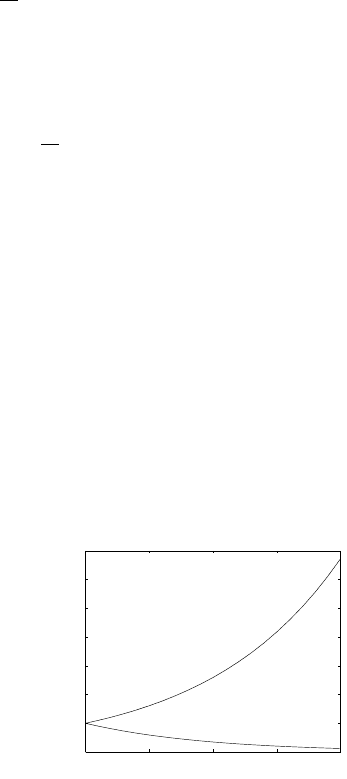
• If λ
i
is positive, λ
t
i
produces ex-
ponential growth if λ>1and
exponential decay if λ<1.
0 5 10 15 20
0
1
2
3
4
5
6
7
t
λ
t
λ = 1.1
λ = 0.9
7.1. Solution of the Projection Equation 153
• If −1 <λ
i
< 0, then λ
t
i
exhibits
damped oscillations with a period
equal to 2.
0 5 10 15 20 25 30 35 40
−1
−0.8
−0.6
−0.4
−0.2
0
0.2
0.4
0.6
0.8
1
t
λ
t
λ = −0.9
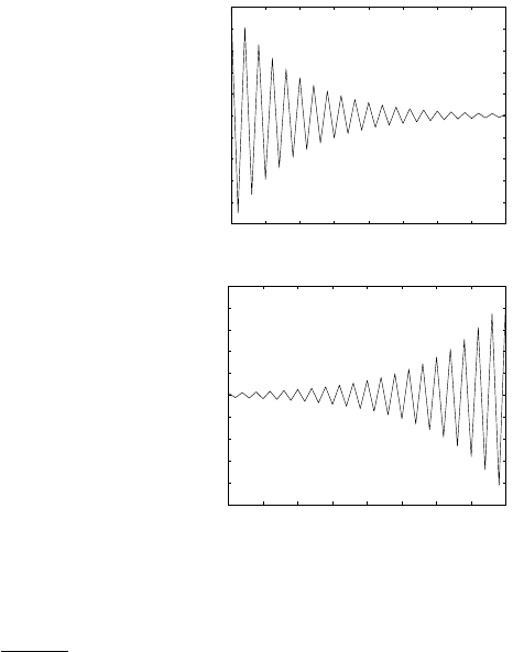
• If λ
i
< −1, then λ
t
i
produces
diverging oscillations with period
2.
0 5 10 15 20 25 30 35 40
−50
−40
−30
−20
−10
0
10
20
30
40
50
t
λ
t
λ = −1.1
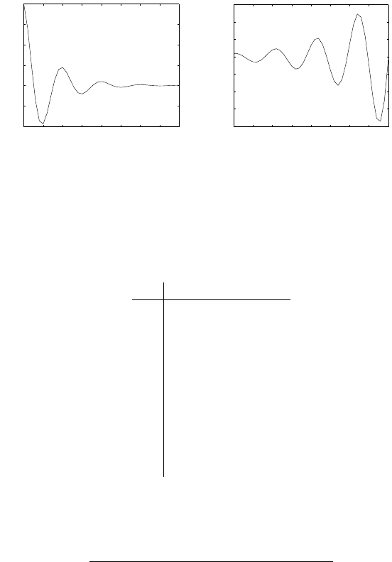
• Complex eigenvalues produce oscillations. Suppose that λ = a + bi,
and write it in polar coordinates,
λ = |λ|(cos θ + i sin θ),
where |λ| =
√
a
2
+ b
2
is the magnitude of λ and θ = tan
−1
(b/a)isthe
angle formed by λ in the complex plane. Raising λ to the tth power
yields
λ
t
= |λ|
t
(cos θt + i sin θt). (7.1.31)
Complex eigenvalues come in complex conjugate pairs, so
¯
λ = a − bi
will also be an eigenvalue. The solution to the projection equation
will thus contain terms of the form
λ
t
+
¯
λ
t
= |λ|
t
2cosθt. (7.1.32)
Thus, as a complex eigenvalue is raised to higher and higher powers,
its magnitude |λ|
t
increases or decreases exponentially, depending on
whether |λ| is greater or less than 1. Its angle in the complex plane
increases by θ each time step, completing an oscillation with a period
of 2π/θ.
154 7. Birth and Population Increase from Matrix Population Models
0 5 10 15 20 25 30 35 40
−1
−0.5
0
0.5
1
1.5
2
t
λ
t
+ (conj λ)
t
λ = 0.7 + 0.5 i
0 5 10 15 20 25 30 35 40
−40
−30
−20
−10
0
10
20
30
t
λ
t
+ (conj λ)
t
λ = 0.9 + 0.6 i
Regardless of whether λ
i
is real or complex, the boundary between
population increase and population decrease comes at |λ
i
| =1.
Example 7.2 An age-classified population
Keyfitz and Flieger (1971) give an age-classified matrix, with 5-year
age classes and a projection interval of 5 years, for the United States
population in 1966. The entries are
i
F
i
P
i
1 0 0.99670
2
0.00102 0.99837
3
0.08515 0.99780
4
0.30574 0.99672
5
0.40002 0.99607
6
0.28061 0.99472
7
0.15260 0.99240
8
0.06420 0.98867
9
0.01483 0.98274
10
0.00089
The eigenvalues of this matrix (in decreasing order of absolute mag-
nitude), their magnitudes, and the angle θ (as a fraction of π) defined
in the complex plane by each are
λ
i
|λ
i
| θ/π
1.0498 1.0498 0.0000
0.3112 + 0.7442i 0.8067 0.3739
0.3112 − 0.7442i 0.8067 −0.3739
−0.3939 + 0.3658i 0.5375 −0.7618
−0.3939 − 0.3658i 0.5375 0.7618
0.0115 + 0.5221i 0.5223 0.4930
0.0115 − 0.5221i 0.5223 −0.4930
−0.4112 + 0.1204i 0.4284 −0.9093
−0.4112 − 0.1204i 0.4284 0.9093
−0.0852 0.0852 1.0000