Jacques I. Mathematics for Economics and Business

Подождите немного. Документ загружается.

which gives

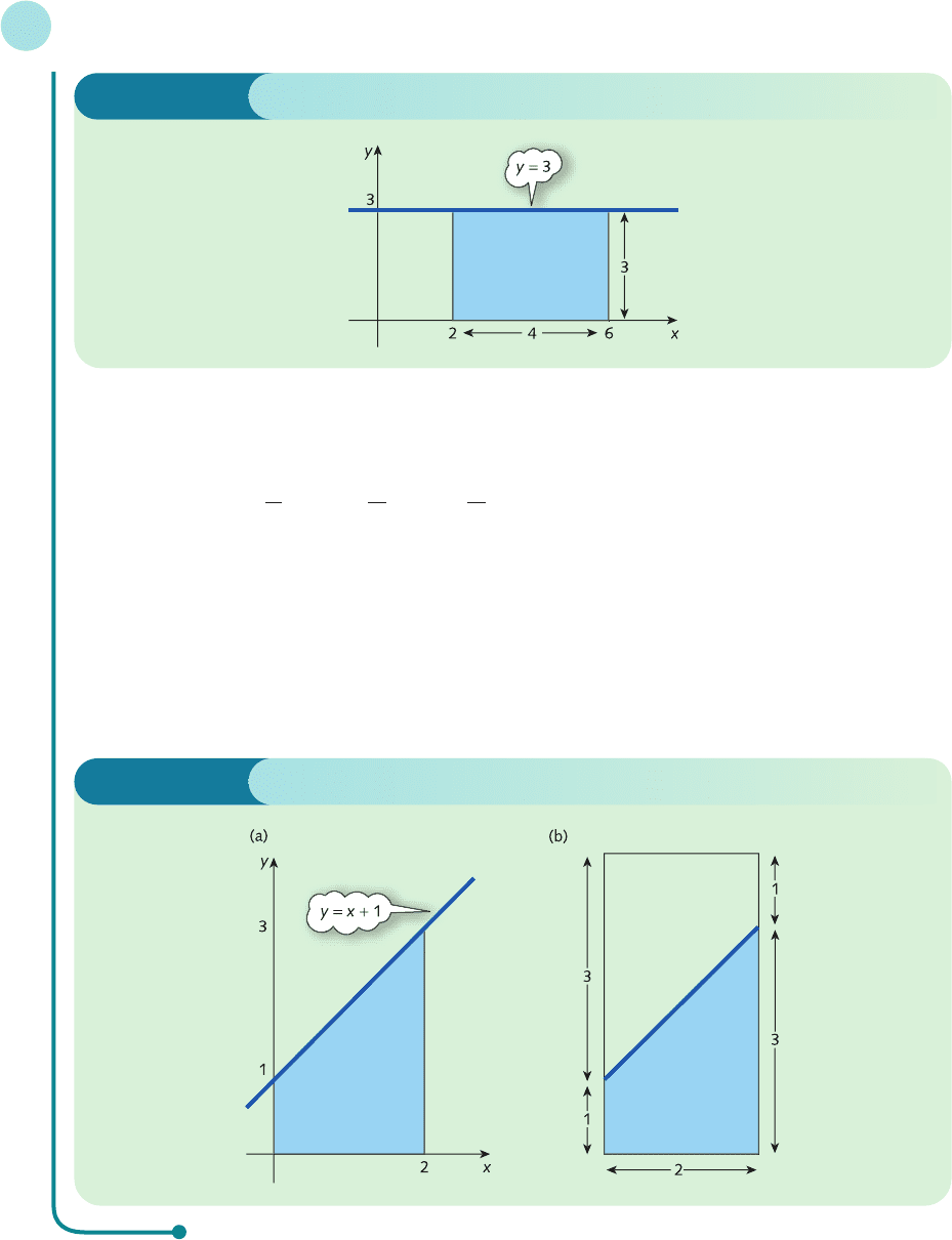
area = 4 × 3 = 12 ✓

(b)



(x + 1)dx = + x

=+2 −+0 = 4

Again this value can be conﬁrmed graphically. Figure 6.5(a) shows the region under the graph of

y = x + 1 between x = 0 and x = 2. This can also be regarded as one-half of the rectangle illustrated in

Figure 6.5(b). This rectangle has a base of 2 units and a height of 4 units, so has area

2 × 4 = 8

The area of the region shown in Figure 6.5(a) is therefore

× 8 = 4 ✓

Integration

440

Figure 6.5

Figure 6.4

In this example we deliberately chose two very simple functions so that we could demon-

strate the fact that deﬁnite integrals really do give the areas under graphs. The beauty of the

integration technique, however, is that it can be used to calculate areas under quite complicated

functions for which alternative methods would fail to produce the exact value.

MFE_C06b.qxd 16/12/2005 11:21 Page 440

To illustrate the applicability of deﬁnite integration we concentrate on four topics:

 consumer’s surplus

 producer’s surplus

 investment ﬂow

 discounting.

We consider each of these in turn.

6.2.1 Consumer’s surplus

The demand function, P = f(Q), sketched in Figure 6.6, gives the different prices that con-

sumers are prepared to pay for various quantities of a good. At Q = Q

the price P = P

. The

total amount of money spent on Q

goods is then Q

, which is given by the area of the rect-

angle OABC. Now, P

is the price that consumers are prepared to pay for the last unit that they

buy, which is the Q

th good. For quantities up to Q

they would actually be willing to pay the

higher price given by the demand curve. The shaded area BCD therefore represents the beneﬁt

to the consumer of paying the ﬁxed price of P

and is called the consumer’s surplus, CS. The

value of CS can be found by observing that

area BCD = area OABD − area OABC

6.2 • Definite integration

441

Figure 6.6

Practice Problem

1 Evaluate the following definite integrals:

(a)



dx (b)



(2x − 1)dx (c)



− x + 1)dx (d)



MFE_C06b.qxd 16/12/2005 11:21 Page 441

The area OABD is the area under the demand curve P = f(Q), between Q = 0 and Q = Q

, and

so is equal to



f(Q)dQ

The region OABC is a rectangle with base Q

and height P

area OABC = Q

Hence

CS =



f(Q)dQ − Q

Integration

442

Practice Problem

2 Find the consumer’s surplus at Q = 8 for the demand function

P = 100 − Q

Example

Find the consumer’s surplus at Q = 5 for the demand function

P = 30 − 4Q

Solution

In this case

f(Q) = 30 − 4Q

and Q

= 5. The price is easily found by substituting Q = 5 into

P = 30 − 4Q

to get

= 30 − 4(5) = 10

The formula for consumer’s surplus

CS =



f(Q)dQ − Q

gives

CS =



(30 − 4Q)dQ − 5(10)

= [30Q − 2Q

]

− 50

= [30(5) − 2(5)

] − [30(0) − 2(0)

] − 50

= 50

MFE_C06b.qxd 16/12/2005 11:21 Page 442

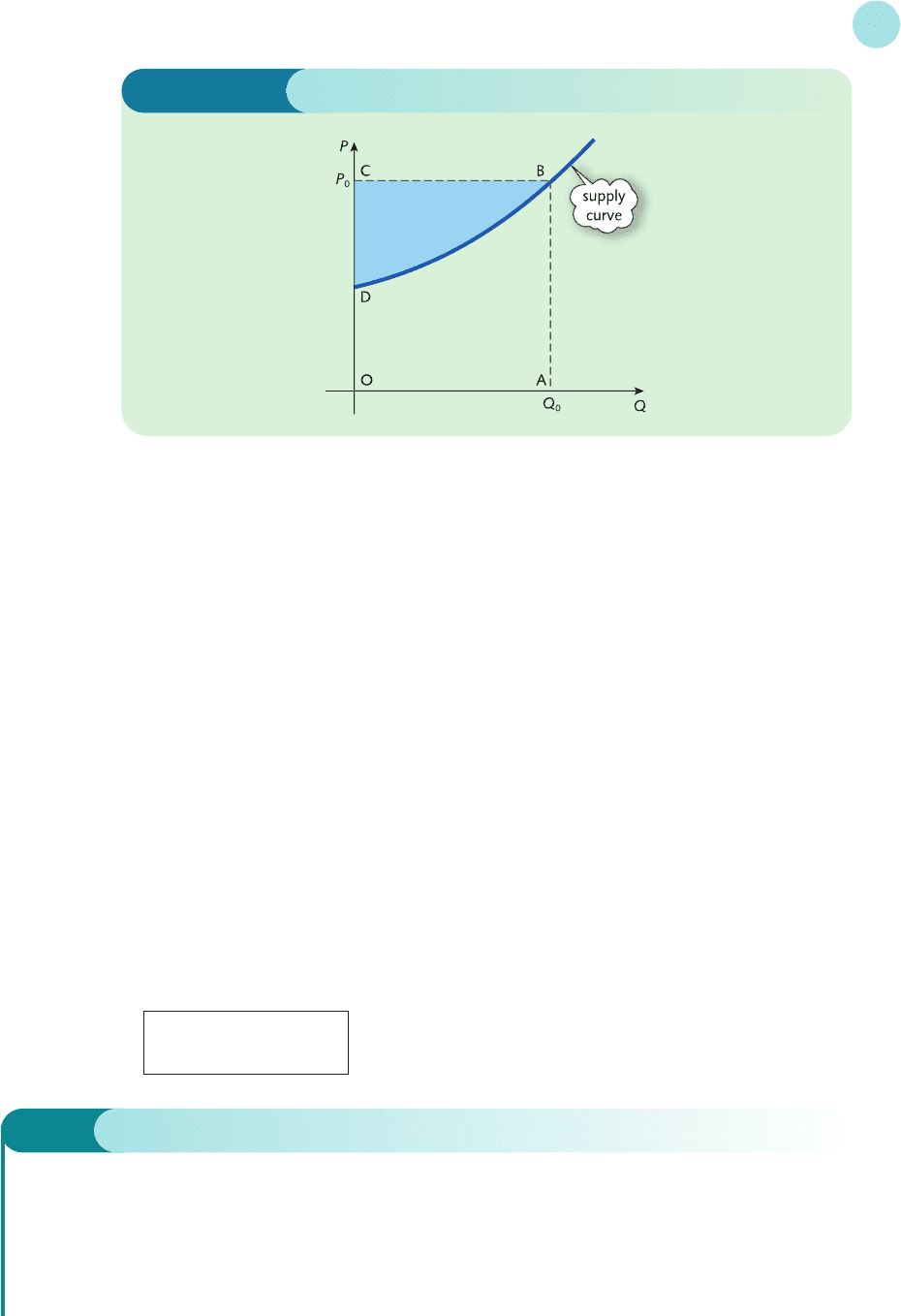
6.2.2 Producer’s surplus

The supply function, P = g(Q), sketched in Figure 6.7 gives the different prices at which pro-

ducers are prepared to supply various quantities of a good. At Q = Q

the price P = P

. Assuming

that all goods are sold, the total amount of money received is then Q

, which is given by the

area of the rectangle OABC.

Now, P

is the price at which the producer is prepared to supply the last unit, which is the

th good. For quantities up to Q

they would actually be willing to accept the lower price given

by the supply curve. The shaded area BCD therefore represents the beneﬁt to the producer of

selling at the ﬁxed price of P

and is called the producer’s surplus, PS. The value of PS is found

by observing that

area BCD = area OABC − area OABD

The region OABC is a rectangle with base Q

and height P

, so

area OABC = Q

The area OABD is the area under the supply curve P = g(Q), between Q = 0 and Q = Q

, and so

is equal to



g(Q)dQ

Hence

PS = Q

−



g(Q)dQ

6.2 • Definite integration

443

Figure 6.7

Example

Given the demand function

P = 35 − Q

and supply function

P = 3 + Q

ﬁnd the producer’s surplus assuming pure competition.



MFE_C06b.qxd 16/12/2005 11:21 Page 443

Solution

On the assumption of pure competition, the price is determined by the market. Before we can calculate the

producer’s surplus we therefore need to ﬁnd the market equilibrium price and quantity. Denoting the com-

mon value of Q

and Q

by Q, the demand and supply functions are

P = 35 − Q

and

P = 3 + Q

so that

35 − Q

= 3 + Q

(both sides are equal to P)

35 − 2Q

= 3 (subtract Q

from both sides)

−2Q

=−32 (subtract 35 from both sides)

= 16 (divide both sides by −2)

which has solution Q =±4. We can obviously ignore the negative solution because it does not make

economic sense. The equilibrium quantity is therefore equal to 4. The corresponding price can be found by

substituting this into either the demand or the supply equation. From the demand equation we have

= 35 − (4)

= 19

The formula for the producer’s surplus,

PS = Q

−



g(Q)dQ

gives

PS = 4(19) −



(3 + Q

)dQ

= 76 − 3Q +

= 76 − {[3(4) +

/3(4)

] − [3(0) −

/3(0)

]}

= 42

Integration

444

Practice Problem

3 Given the demand equation

P = 50 − 2Q

and supply equation

P = 10 + 2Q

calculate

(a) the consumer’s surplus

(b) the producer’s surplus

assuming pure competition.

MFE_C06b.qxd 16/12/2005 11:21 Page 444

6.2.3 Investment ﬂow

Net investment, I, is deﬁned to be the rate of change of capital stock, K, so that

I =

Here I(t) denotes the ﬂow of money, measured in dollars per year, and K(t) is the amount of

capital accumulated at time t as a result of this investment ﬂow and is measured in dollars.

Given a formula for capital stock in terms of time, we simply differentiate to ﬁnd net invest-

ment. Conversely, if we know the net investment function then we integrate to ﬁnd the capital

stock. In particular, to calculate the capital formation during the time period from t = t

t = t

we evaluate the deﬁnite integral



I(t )dt

6.2 • Definite integration

445

Example

If the investment ﬂow is

I(t) = 9000 t

calculate

(a) the capital formation from the end of the ﬁrst year to the end of the fourth year

(b) the number of years required before the capital stock exceeds $100 000.

Solution

(a) In this part we need to calculate the capital formation from t = 1 to t = 4, so we evaluate the deﬁnite

integral



9000 t dt= 9000



1/2

= 9000 t

3/2

= 9000 (4)

3/2

− (1)

3/2

= 9000 −

= $42 000

(b) In this part we need to calculate the number of years required to accumulate a total of $100 000. After

T years the capital stock is



9000 t dt = 9000



1/ 2

We want to ﬁnd the value of T so that

9000



1/ 2

dt = 100 000



MFE_C06b.qxd 16/12/2005 11:21 Page 445

The integral is easily evaluated as

9000 t

3/2

= 9000 T

3/2

− (0)

3/2

= 6000T

3/2

so T satisﬁes

6000T

3/2

= 100 000

This non-linear equation can be solved by dividing both sides by 6000 to get

3/2

= 16.67

and then raising both sides to the power of

, which gives

T = 6.5

The capital stock reaches the $100 000 level about halfway through the seventh year.

Integration

446

Practice Problem

4 If the net investment function is given by

I(t) = 800t

1/3

calculate

(a) the capital formation from the end of the first year to the end of the eighth year

(b) the number of years required before the capital stock exceeds $48 600.

Example

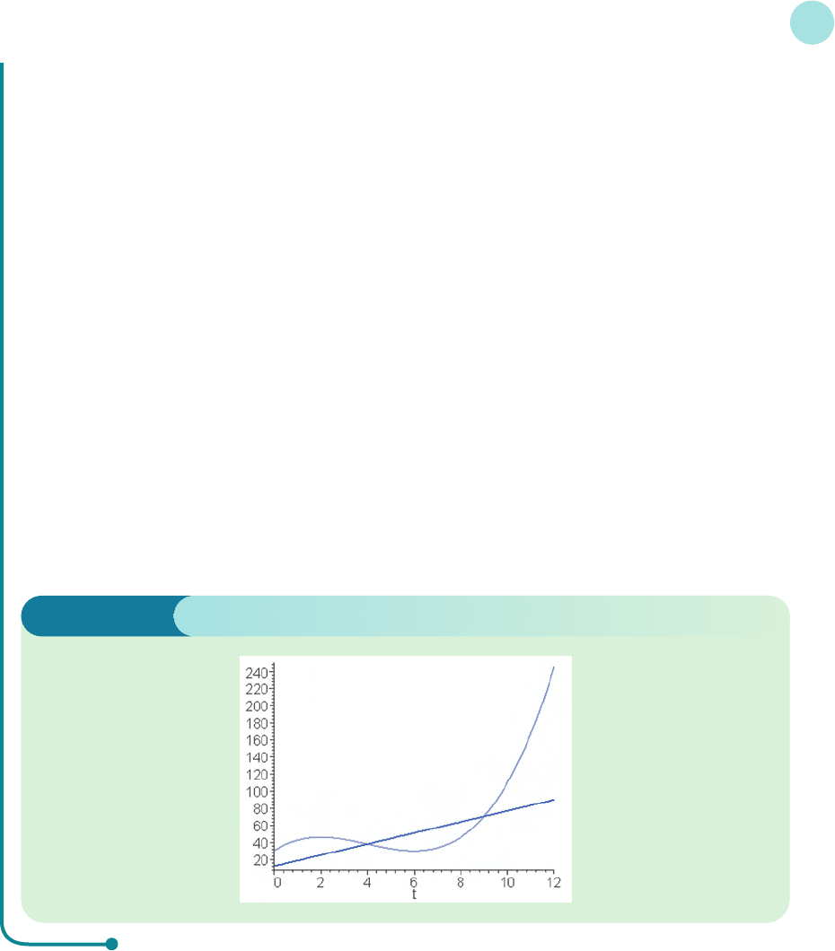
During the next year, a ﬁrm’s revenue and cost ﬂows, measured in thousands of dollars per month, are to

be modelled by

r(t) = 0.5t

− 6t

+ 18t + 30 and c(t) = 6.5t + 12

respectively.

(1) Evaluate the deﬁnite integrals

(a)



(r − c)dt (b)



(r − c)dt

(2) Plot a graph of r(t) and c(t) on the same diagram and hence interpret the values obtained in part (1).

Solution

(1) We begin by naming these expressions r and c by typing

>r:=0.5*t^3–6*t^2+18*t+30;

and

>c:=6.5*t+12;

MAPLE

MFE_C06b.qxd 16/12/2005 11:21 Page 446

(a) To evaluate the deﬁnite integral ∫

(r − c)dt, we use the instruction int as before, except that we

now specify the limits, 0 and 4. We type

>int(r-c,t=0..4);

which gives the answer

(b) Similarly, the second integral is evaluated by editing the instruction as:

>int(r-c,t=4..9);

which gives

–78.125

(2) To plot both r and c on the same diagram, type

>plot({r,c},t=0..12);

The result is sketched in Figure 6.8.

Now, r(t) represents the rate of change of revenue with respect to time, so the revenue itself is the area

under the graph of r(t). Similarly, the area under the graph of c(t) determines the total cost. Hence the

area between the two curves gives the predicted proﬁt during that time period. Figure 6.8 shows that

between t = 0 and t = 4 revenue exceeds costs, so the ﬁrm is likely to make a positive proﬁt of $68 000.

On the other hand, between t = 4 and t = 9 the graph of c(t) lies above that of r(t), which explains why

the value of the integral is negative. During this period the ﬁrm is expected to make a loss of $78 125.

6.2 • Definite integration

447

6.2.4 Discounting

In Chapter 3 the formula

P = Se

−rt / 100

was used to calculate the present value, P, when a single future value, S, is discounted at r%

interest continuously for t years. We also discussed the idea of an annuity. This is a fund that

provides a series of discrete regular payments and we showed how to calculate the original

lump sum needed to secure these payments for a prescribed number of years. This amount is

Figure 6.8

MFE_C06b.qxd 16/12/2005 11:21 Page 447

called the present value of the annuity. If the fund is to provide a continuous revenue stream

for n years at an annual rate of S dollars per year then the present value can be found by eval-

uating the deﬁnite integral

P =



−rt / 100

Integration

448

Practice Problem

5 Calculate the present value of a continuous revenue stream for 10 years at a constant rate of $5000

per year if the discount rate is 6%.

Example

Calculate the present value of a continuous revenue stream for 5 years at a constant rate of $1000 per year

if the discount rate is 9%.

Solution

The present value is found from the formula

P =



−rt/100

with S = 1000, r = 9 and n = 5, so

P =



1000e

− 0.09t

= 1000



− 0.09t

= 1000 − e

− 0.09t

=− [e

− 0.09t

]

=− (e

− 0.45

− 1)

= $4026.35

1000

0.09

1000

0.09

MFE_C06b.qxd 16/12/2005 11:21 Page 448

6.2 • Definite integration

449

Consumer’s surplus The excess cost that a person would have been prepared to pay for

goods over and above what is actually paid.

Deﬁnite integral The number ∫

f(x)dx which represents the area under the graph of f (x)

between x = a and x = b.

Limits of integration The numbers a and b which appear in the deﬁnite integral, ∫

f(x)dx.

Net investment Rate of change of capital stock over time: I = dK/dt.

Producer’s surplus The excess revenue that a producer has actually received over and

above the lower revenue that it was prepared to accept for the supply of its goods.

Key Terms

Practice Problems

6 Find the area under the graph of

f(x) = 4x

− 3x

+ 4x + 2

between x = 1 and x = 2.

7 Evaluate each of the following definite integrals:

(a)



dx (b)



−2

By sketching a rough graph of the cube function between and x =−2 and 2, suggest a reason for your

answer to part (b). What is the actual area between the x axis and the graph of y = x

over this range?

8 (Maple)

(a) Plot a graph of y = on 1 ≤ x ≤ 30.

Evaluate



dx in the cases when N is 2, 20 and 200.

What do these results suggest about the value of



∞

dx?

(b) Repeat part (a) for the function y = .

9 (Maple)

(a) Plot a graph of y = on 0.01 ≤ x ≤ 1.

Evaluate



dx in the cases when N is 0.1, 0.01 and 0.001.

What do these results suggest about the value of



dx?

(b) Repeat part (a) for the function y = .



MFE_C06b.qxd 16/12/2005 11:21 Page 449