Jackson S.L. Research Methods and Statistics: A Critical Thinking Approach
Подождите немного. Документ загружается.


172
■ ■
CHAPTER 7
The z Test: What It Is and What It Does
The z test is a parametric statistical test that allows us to test the null hypoth-
esis for a single sample when the population variance is known. This proce-
dure allows us to compare a sample with a population to assess whether the
sample differs significantly from the population. If the sample was drawn
randomly from a certain population (children in academic after-school pro-
grams), and we observe a difference between the sample and a broader pop-
ulation (all children), we can then conclude that the population represented
by the sample differs significantly from the comparison population. Let’s
return to our previous example and assume that we have actually collected
IQ scores from 75 students enrolled in academic after-school programs. We
want to determine whether the sample of children in academic after-school
programs represents a population with a mean IQ higher than the mean IQ
of the general population of children. We already know (100) and (15)
for the general population of children. The null and alternative hypotheses
for a one-tailed test are
H
0
:
0
1
, or
academic program
general population
H
a
:
0
1
, or
academic program
general population
z test A parametric inferen-
tial statistical test of the null
hypothesis for a single sample
where the population variance
is known.
z test A parametric inferen-
tial statistical test of the null
hypothesis for a single sample
where the population variance
is known.
IN REVIEW Inferential Statistical Tests
CONCEPT DESCRIPTION EXAMPLE
Parametric Inferential Inferential statistical procedures that require z test
Statistics certain assumptions about the parameters t test
of the population represented by the sample
data, such as knowing and and that the
distribution is normal
Most often used with interval or ratio data
Nonparametric Inferential Inferential procedures that do not require Chi-square tests
Statistics assumptions about the parameters of the Wilcoxon tests
population represented by the sample data; (Discussed
and are not needed, and the underlying in Chapter 9)
distribution does not have to be normal
Most often used with ordinal or nominal data
CRITICAL
THINKING
CHECK
7.2
1. How do inferential statistics differ from descriptive statistics?
2. How does single-sample research involve the use of hypothesis
testing? In other words, in a single-group design, what hypothesis
is tested?
10017_07_ch7_p163-201.indd 172 2/1/08 1:24:49 PM
Hypothesis Testing and Inferential Statistics
■ ■
173
In Chapter 5, you learned how to calculate a z-score for a single data
point (or a single individual’s score). To review, the formula for a z-score is
z
X –
_____
Remember that a z-score tells us how many standard deviations above
or below the mean of the distribution an individual score falls. When
using the z test, however, we are not comparing an individual score with
the population mean. Instead, we are comparing a sample mean with
the population mean. We therefore cannot compare the sample mean
with a population distribution of individual scores. We must compare
it instead with a distribution of sample means, known as the sampling
distribution.
The Sampling Distribution
If you are becoming confused, think about it this way: A sampling
distribution is a distribution of sample means based on random samples
of a fixed size from a population. Imagine that we have drawn many dif-
ferent samples of the same size (say, 75) from the population (children on
whom we can measure IQ). For each sample that we draw, we calculate
the mean; then we plot the means of all the samples. What do you think
the distribution will look like? Most of the sample means will probably be
similar to the population mean of 100. Some of the sample means will be
slightly lower than 100; some will be slightly higher than 100; and others
will be right at 100. A few of the sample means, however, will not be similar
to the population mean. Why? Based on chance, some samples will contain
some of the rare individuals with either very high IQ scores or very low IQ
scores. Thus, the means for these samples will be much higher than 100 or
much lower than 100. Such samples, however, will be few in number. Thus,
the sampling distribution (the distribution of sample means) will be normal
(bell-shaped), with most of the sample means clustered around 100 and a
few sample means in the tails or the extremes. Therefore, the mean for the
sampling distribution will be the same as the mean for the distribution of
individual scores (100).
The Standard Error of the Mean
Here is a more difficult question: Will the standard deviation of the sam-
pling distribution, known as the standard error of the mean, be the same
as that for a distribution of individual scores? We know that 15 for the
distribution of individual IQ test scores. Will the variability in the sampling
distribution be as great as it is in a distribution of individual scores? Let’s
think about it. The sampling distribution is a distribution of sample means.
In our example, each sample has 75 people in it. Now, the mean for a sam-
ple of 75 people can never be as low or as high as the lowest or highest
sampling distribution
A distribution of sample means
based on random samples of a
fixed size from a population.
sampling distribution
A distribution of sample means
based on random samples of a
fixed size from a population.
standard error of the mean
The standard deviation of the
sampling distribution.
standard error of the mean
The standard deviation of the
sampling distribution.
10017_07_ch7_p163-201.indd 173 2/1/08 1:24:50 PM
174
■ ■
CHAPTER 7
individual score. Why? Most people have IQ scores around 100. This means
that in each of the samples, most people will have scores around 100. A few
people will have very low scores, and when they are included in the sample,
they will pull down the mean for that sample. A few others will have very
high scores, and these scores will raise the mean for the sample in which
they are included. A few people in a sample of 75, however, can never pull
the mean for the sample as low as a single individual’s score might be or as
high as a single individual’s score might be. For this reason, the standard
error of the mean (the standard deviation of the sampling distribution) can
never be as large as (the standard deviation for the distribution of indi-
vidual scores).
How does this relate to the z test? A z test uses the mean and standard
deviation of the sampling distribution to determine whether the sample
mean is significantly different from the population mean. Thus, we need to
know the mean () and the standard error of the mean (
X
) for the sampling
distribution. We have already said that for the sampling distribution is
the same as for the distribution of individual scores—100. How will we
determine what
X
is? To find the standard error of the mean, we need to
draw a number of samples from the population, determine the mean for
each sample, and then calculate the standard deviation for this distribution
of sample means. This is hardly feasible. Luckily for us, there is a means of
finding the standard error of the mean without doing all of this. This is based
on the central limit theorem. The central limit theorem is a precise descrip-
tion of the distribution that would be obtained if you selected every possible
sample, calculated every sample mean, and constructed the distribution
of sample means. The central limit theorem states that for any population
with mean and standard deviation , the distribution of sample means for
sample size N will have a mean of and a standard deviation of /
__
N and
will approach a normal distribution as N approaches infinity. Thus, accord-
ing to the central limit theorem, to determine the standard error of the mean
(the standard deviation for the sampling distribution), we take the standard
deviation for the population () and divide by the square root of the sample
size (
__
N ):
X
____
__
N
We can now use this information to calculate z. The formula for z is
z
X
______
X
where
X sample mean
mean of the sampling distribution
X
standard deviation of the sampling distribution, or standard error
of the mean
central limit theorem
A theorem which states that for
any population with mean
and standard deviation , the
distribution of sample means
for sample size N will have
a mean of and a standard
deviation of /
__
N and will
approach a normal distribution
as N approaches infinity.
central limit theorem
A theorem which states that for
any population with mean
and standard deviation , the
distribution of sample means
for sample size N will have
a mean of and a standard
deviation of /
__
N and will
approach a normal distribution
as N approaches infinity.
10017_07_ch7_p163-201.indd 174 2/1/08 1:24:50 PM

Hypothesis Testing and Inferential Statistics
■ ■
175
Calculations for the One-Tailed z Test
You can see that the formula for a z test represents finding the difference
between the sample mean (
X ) and the population mean () and then divid-
ing by the standard error of the mean (
X
). This will tell us how many
standard deviation units a sample mean is from the population mean, or the
likelihood that the sample is from that population. We already know and
, so we need to find the mean for the sample (
X ) and to calculate
X
based
on a sample size of 75.
Suppose we find that the mean IQ score for the sample of 75 children
enrolled in academic after-school programs is 103.5. We can calculate
X
based on knowing the sample size and :
X
____
__
N
15
_____
___
75
15
____
8.66
1.73
We now use
X
(1.73) in the z-test formula:
z
X
______
X
103.5 100
___________
1.73
3.5
____
1.73
2.02
CRITICAL
THINKING
CHECK
7.3
1. Explain how a sampling distribution differs from a distribution of
individual scores.
2. Explain the difference between
X
and .
3. How is a z test different from a z-score?
The z Test (Part I) IN REVIEW
CONCEPT DESCRIPTION USE
Sampling Distribution A distribution of sample means where Used for comparative purposes for
each sample is the same size (N) z tests—a sample mean is compared
with the sampling distribution to
assess the likelihood that the sample
is part of the sampling distribution
Standard Error of the The standard deviation of a sampling Used in the calculation of z
Mean (
X
) distribution, determined by dividing
by
__
N
z Test Indication of the number of standard An inferential test that compares
deviation units the sample mean is from a sample mean with the sampling
the mean of the sampling distribution distribution to determine the
likelihood that the sample is part
of the sampling distribution
10017_07_ch7_p163-201.indd 175 2/1/08 1:24:50 PM
176
■ ■
CHAPTER 7
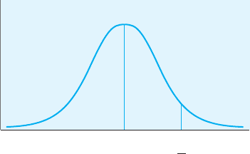
Interpreting the One-Tailed z Test
Figure 7.1 shows where the sample mean of 103.5 lies with respect to the
population mean of 100. The z-test score of 2.02 can be used to test our
hypothesis that the sample of children in academic after-school programs
represents a population with a mean IQ higher than the mean IQ for the gen-
eral population. To do this, we need to determine whether the probability is
high or low that a sample mean as large as 103.5 would be found from this
sampling distribution. In other words, is a sample mean IQ score of 103.5 far
enough away from, or different enough from, the population mean of 100
for us to say that it represents a significant difference with an alpha level
of .05 or less?
How do we determine whether a z-score of 2.02 is statistically signifi-
cant? Because the sampling distribution is normally distributed, we can use
the area under the normal curve (Table A.2 in Appendix A). When we dis-
cussed z-scores in Chapter 5, we saw that Table A.2 provides information on
the proportion of scores falling between and the z-score and the proportion
of scores beyond the z-score. To determine whether a z test is significant, we
can use the area under the curve to determine whether the chance of a given
score occurring is 5% or less. In other words, is the score far enough away
from (above or below) the mean that only 5% or less of the scores are as far
or farther away?
Using Table A.2, we find that the z-score that marks off the top 5% of
the distribution is 1.645. This is referred to as the z critical value, or z
cv
—the
value of a test statistic that marks the edge of the region of rejection in a
sampling distribution. The region of rejection is the area of a sampling dis-
tribution that lies beyond the test statistic’s critical value; when a score falls
within this region, H
0
is rejected. For us to conclude that the sample mean
is significantly different from the population mean, then, the sample mean
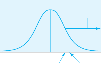
must be at least ±1.645 standard deviations (z units) from the mean. The
critical value of ±1.645 is illustrated in Figure 7.2. The z we obtained for our
sample mean (z
obt
) is 2.02, and this value falls within the region of rejection
for the null hypothesis. We therefore reject H
0
that the sample mean repre-
sents the general population mean and support our alternative hypothesis
that the sample mean represents a population of children in academic after-
school programs whose mean IQ is higher than 100. We make this decision
because the z-test score for the sample is greater than (farther out in the
critical value The value of a
test statistic that marks the edge
of the region of rejection in a
sampling distribution, where
values equal to it or beyond it
fall in the region of rejection.
critical value The value of a
test statistic that marks the edge
of the region of rejection in a
sampling distribution, where
values equal to it or beyond it
fall in the region of rejection.
region of rejection The
area of a sampling distribu-
tion that lies beyond the test
statistic’s critical value; when a
score falls within this region, H
0
is rejected.
region of rejection The
area of a sampling distribu-
tion that lies beyond the test
statistic’s critical value; when a
score falls within this region, H
0
is rejected.
103.5100
Xμ
FIGURE 7.1
The obtained mean
in relation to the
population mean
10017_07_ch7_p163-201.indd 176 2/1/08 1:24:51 PM
Hypothesis Testing and Inferential Statistics
■ ■
177
tail than) the critical value of ±1.645. In APA style (discussed in detail in
Chapter 13), the result is reported as
z (N 75) 2.06, p .05 (one-tailed)
This style conveys in a concise manner the z-score, the sample size, that the
results are significant at the .05 level, and that we used a one-tailed test.
The test just conducted was a one-tailed test because we predicted
that the sample would score higher than the population. What if this were
reversed? For example, imagine I am conducting a study to see whether chil-
dren in athletic after-school programs weigh less than children in the general
population. What are H
0
and H
a
for this example?
H
0
:
0
1
, or
athletic programs
general population
H
a
:
0
1
, or
athletic programs
general population
Assume that the mean weight of children in the general population ()
is 90 pounds, with a standard deviation () of 17 pounds. You take a ran-
dom sample (N 50) of children in athletic after-school programs and find
a mean weight (
X ) of 86 pounds. Given this information, you can test the
hypothesis that the sample of children in athletic after-school programs rep-
resents a population with a mean weight that is lower than the mean weight
for the general population of children.
First, we calculate the standard error of the mean (
X
):
X
____
__
N
17
_____
___
50
17
____
7.07
2.40
Now, we enter
X
into the z-test formula:
z
X
______
X
86 90
_______
2.40
4
____
2.40
1.67
The z-score for this sample mean is 1.67, meaning that it falls 1.67 standard
deviations below the mean. The critical value for a one-tailed test is 1.645
standard deviations. This means the z-score has to be at least 1.645 standard
deviations away from (above or below) the mean to fall in the region of rejec-
tion. In other words, the critical value for a one-tailed z test is ±1.645. Is our
z-score at least that far away from the mean? It is, but just barely. Therefore,
+2.02
Region
of rejection
+1.645
z
obt
z
cv
FIGURE 7.2
The z critical value
and the z obtained
for the z test
example
10017_07_ch7_p163-201.indd 177 2/1/08 1:24:52 PM
178
■ ■
CHAPTER 7
we reject H
0
and accept H
a
—that children in athletic after-school programs
weigh significantly less than children in the general population and hence
represent a population of children who weigh less. In APA style, the result
is reported as
z (N 50) 1.67, p .05 (one-tailed)
Calculations for the Two-Tailed z Test
So far, we have completed two z tests, both one-tailed. Let’s turn now to a
two-tailed z test. Remember that a two-tailed test is also known as a nondi-
rectional test—a test in which the prediction is simply that the sample will
perform differently from the population, with no prediction as to whether
the sample mean will be lower or higher than the population mean.
Suppose that in the previous example, we used a two-tailed rather than
a one-tailed test. We expect the weight of children in athletic after-school
programs to differ from the weight of children in the general population,
but we are not sure whether they will weigh less (because of the activity)
or more (because of greater muscle mass). H
0
and H
a
for this two-tailed test
appear next. See if you can determine what they would be before you con-
tinue reading.
H
0
:
0
1
, or
athletic programs
general population
H
a
:
0
1
, or
athletic programs
general population
Let’s use the same data as before: The mean weight of children in the general
population () is 90 pounds, with a standard deviation () of 17 pounds; for
children in the sample (N 50), the mean weight (
X ) is 86 pounds. Using
this information, we can now test the hypothesis that children in athletic
after-school programs differ in weight from those in the general population.
Notice that the calculations will be exactly the same for this z test; that is,
X
and the z-score will be exactly the same as before. Why? All of the measure-
ments are exactly the same. To review:
X
____
__
N
17
_____
___
50
17
____
7.07
2.40
z
X
______
X
86 90
_______
2.40
4
____
2.40
1.67
Interpreting the Two-Tailed z Test
If we end up with the same z-score, how does a two-tailed test differ from
a one-tailed test? The difference is in the z critical value (z
cv
). In a two-tailed
test, both halves of the normal distribution have to be taken into account.
Remember that with a one-tailed test, z
cv
was ±1.645; this z-score was so far
away from the mean (either above or below) that only 5% of the scores were
beyond it. How does the z
cv
for a two-tailed test differ? With a two-tailed test,
z
cv
has to be so far away from the mean that a total of only 5% of the scores
10017_07_ch7_p163-201.indd 178 2/1/08 1:24:52 PM
Hypothesis Testing and Inferential Statistics
■ ■
179
are beyond it (both above and below the mean). A z
cv
of ±1.645 leaves 5% of
the scores above the positive z
cv
and 5% below the negative z
cv
. If we take
both sides of the normal distribution into account (which we do with a two-
tailed test because we do not predict whether the sample mean will be above
or below the population mean), then 10% of the distribution will fall beyond
the two critical values. Thus, ±1.645 cannot be the critical value for a two-
tailed test because this leaves too much chance (10%) operating.
To determine z
cv
for a two-tailed test, then, we need to find the z-score
that is far enough away from the population mean that only 5% of the
distribution—taking into account both halves of the distribution—is
beyond the score. Because Table A.2 (in Appendix A) represents only half
of the distribution, we need to look for the z-score that leaves only 2.5% of
the distribution beyond it. Then, when we take into account both halves
of the distribution, 5% of the distribution will be accounted for (2.5%
2.5% 5%). Can you determine this z-score using Table A.2? If you find that
it is ±1.96, you are correct. This is the z-score that is far enough away from
the population mean (using both halves of the distribution) that only 5% of
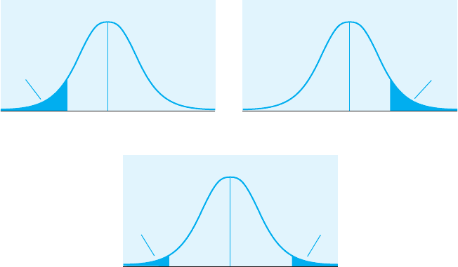
the distribution is beyond it. The critical values for both one- and two-tailed
tests are illustrated in Figure 7.3.
Okay, what do we do with this critical value? We use it exactly the
same way we used z
cv
for a one-tailed test. In other words, z
obt
has to be
as large as or larger than z
cv
for us to reject H
0
. Is our z
obt
as large as or
larger than ±1.96? No, our z
obt
is 1.67. We therefore fail to reject H
0
and
conclude that the weight of children in athletic after-school programs
does not differ significantly from the weight of children in the general
population.
With exactly the same data (sample size, , ,
X , and
X
), we rejected H
0
using a one-tailed test and failed to reject H
0
with a two-tailed test. How can
this be? The answer is that a one-tailed test is statistically a more powerful
μ
null
z
critical
= –1.645
α = .05
μ
null
z
critical
= –1.96 z
critical
= +1.96
.025
.025
μ
null
z
critical
= +1.645
α = .05
FIGURE 7.3
Regions of rejection
and critical values
for one-tailed versus
two-tailed tests
10017_07_ch7_p163-201.indd 179 2/1/08 1:24:53 PM
180
■ ■
CHAPTER 7
test than a two-tailed test. Statistical power refers to the probability of cor-
rectly rejecting a false H
0
. With a one-tailed test, we are more likely to reject
H
0
because z
obt
does not have to be as large (as far away from the popula-
tion mean) to be considered significantly different from the population
mean. (Remember, z
cv
for a one-tailed test is ±1.645, but for a two-tailed test,
it is ±1.96.)
Statistical Power
Let’s think back to the discussion of Type I and II errors. We said that to
reduce the risk of a Type I error, we need to lower the alpha level—for exam-
ple, from .05 to .01. We also noted, however, that lowering the alpha level
increases the risk of a Type II error. How, then, can we reduce the risk of a
Type I error but not increase the risk of a Type II error? As we just noted,
a one-tailed test is more powerful—we do not need as large a z
cv
to reject
H
0
. Here, then, is one way to maintain an alpha level of .05 but increase
our chances of correctly rejecting H
0
. Of course, ethically we cannot simply
choose to adopt a one-tailed test for this reason. The one-tailed test should be
adopted only because we truly believe that the sample will perform above
(or below) the mean.
By what other means can we increase statistical power? Look back at
the z-test formula. We know that the larger z
obt
is, the greater the chance
that it will be significant (as large as or larger than z
cv
), and we can therefore
reject H
0
. What could we change in our study that might increase z
obt
? Well,
if the denominator in the z formula were a smaller number, then z
obt
would
be larger and more likely to fall in the region of rejection. How can we make
the denominator smaller? The denominator is
X
. Do you remember the
formula for
X
?
X
____
__
N
It is very unlikely that we can change or influence the standard deviation of
the population (). The part of the
X
formula that we can influence is the
sample size (N).
If we increase the sample size, what will happen to
X
? Let’s see. We can
use the same example as before: a two-tailed test with all of the same meas-
urements. The only difference will be the sample size. Thus, the null and
alternative hypotheses are
H
0
:
0
1
, or
athletic programs
general population
H
a
:
0
1
, or
athletic programs
general population
The mean weight () of children in the general population is once again
90 pounds with a standard deviation () of 17 pounds, and the sample
of children in after-school programs again has a mean weight (
X ) of
86 pounds. The only difference is the sample size. In this case, our sample
statistical power The prob-
ability of correctly rejecting a
false H
0
.
statistical power The prob-
ability of correctly rejecting a
false H
0
.
10017_07_ch7_p163-201.indd 180 2/1/08 1:24:53 PM
Hypothesis Testing and Inferential Statistics
■ ■
181
has 100 children in it. Let’s test the hypothesis (conduct the z test) for
these data:
X
17
______
____
100
17
___
10
1.7
z
86 90
_______
1.70
4
____
1.70
2.35
Do you see what happened when we increased the sample size? The stand-
ard error of the mean (
X
) decreased (we will discuss why in a minute),
and z
obt
increased—in fact, it increased to the extent that we can now reject
H
0
with this two-tailed test because our z
obt
of 2.35 is larger than the z
cv
of ±1.96. Therefore, another way to increase statistical power is to increase
the sample size.
Why does increasing the sample size decrease
X
? Well, you can see
why based on the formula, but let’s think back to our earlier discus-
sion about
X
. We said that it is the standard deviation of a sampling
distribution—a distribution of sample means. If you recall the IQ example
we used in our discussion of
X
and the sampling distribution, we said that
100 and 15. We discussed what
X
is for a sampling distribution
in which each sample mean is based on a sample size of 75. We further noted
that
X
is always smaller (has less variability) than because it represents
the standard deviation of a distribution of sample means, not a distribution
of individual scores. What, then, does increasing the sample size do to
X
?
If each sample in the sampling distribution has 100 people in it rather than 75,
what do you think this will do to the distribution of sample means? As we
noted earlier, most people in a sample will be close to the mean (100), with
only a few people in each sample representing the tails of the distribution.
If we increase the sample size to 100, we will have 25 more people in each
sample. Most of them will probably be close to the population mean of 100;
therefore, each sample mean will probably be closer to the population mean
of 100. Thus, a sampling distribution based on samples of N 100 rather
than N 75 will have less variability, which means that
X
will be smaller. In
sum, as the sample size increases, the standard error of the mean decreases.
Assumptions and Appropriate Use of the z Test
As noted earlier in the chapter, the z test is a parametric inferential statistical
test for hypothesis testing. Parametric tests involve the use of parameters,
or population characteristics. With a z test, the parameters, such as and ,
are known. If they are not known, the z test is not appropriate. Because the z
test involves the calculation and use of a sample mean, it is appropriate for
use with interval or ratio data. In addition, because we use the area under
the normal curve (see Table A.2 in Appendix A), we are assuming that the
distribution of random samples is normal. Small samples often fail to form a
normal distribution. Therefore, if the sample size is small (N 30), the z test
may not be appropriate. In cases where the sample size is small, or where
is not know, the appropriate test is the t test, discussed later in the text.
10017_07_ch7_p163-201.indd 181 2/1/08 1:24:54 PM