Iozzo Renato V. Proteoglycan Protocols

Подождите немного. Документ загружается.

418 Forsten and Nugent

3. Method

3.1. Experimental Protocol

1. Label and arrange 0.5-mL microcentrifuge tubes—1 per sample, 3 per condition.

2. Prepare incubation buffer—Buffer may be made in advance and filter-sterilized for later

use. No degassing is needed.

3. Add the needed incubation buffer to each vial—the volume should be 0.2 mL minus the

volume of

125

I-bFGF, inhibitor, and E-HS needed. Controls should be conducted with

vials containing only

125

I-bFGF, and

125

I-bFGF and the inhibitors, to determine the

non-proteoglycan–mediated adsorption of

125

I-bFGF to the filter. These values should be

substrated from the experimental points with E-HS to determine the level of

125

I-bFGF

bound to E-HS.

4. Add the E-HS, inhibitor, and

125

I-bFGF in that order. As a standard assay we have used

40 ng of E-HS and 0.2 ng of

125

I-bFGF in a final volume of 0.2 mL. Under these condi-

tions greater than 80% of the E-HS is retained with and without bFGF addition, and only

~5% of the bFGF will adsorb to the filter nonspecifically. Initial experiments should be

conducted with a range of

125

I-bFGF concentrations to determine the binding affinity and

capacity of each E-HS preparation before inhibitor competition data can be analyzed.

After each addition of

125

I-bFGF, vortex gently to mix and place in an incubation rack. If

the assay is done at a temperature other than room temperature (25°C), be sure that the

buffers are preequilibrated at the desired temperature and that vials are placed immedi-

ately in a temperature equilibrated rack.

5. Incubate for desired time (generally 60 min to reach a steady state in bound versus

unbound bFGF).

6. If incubation is shorter then 30 min, the cationic membrane should be prepared prior to

incubation (steps 3–5). The membrane is cut to fit the apparatus (cover all holes) and then

incubated on a rocking platform for at least 20 min in incubation buffer. Longer incuba-

tions (up to 1 h) do not adversely affect the assay.

7. The membrane is placed on the dot-blot apparatus and the top plate is tightened using a

criss-cross pattern. The apparatus is attached to a vacuum pump (GAST, model ROA-

P131-AA, Manufacturing Corp., Benton Harbor, MI) and the apparatus tightened again

under vacuum. Experiments should be done under a 25 mmHg vacuum.

8. Close off the apparatus to the vacuum and, using a multipipeter, add 0.2 mL of incubation

buffer to each well.

9. When the incubation is within 30 s of completion, turn on the vacuum and pull the wash

buffer through the membrane. Add samples (0.2 mL/well) in sets of three. Wash each

well of the triplicate set once with 0.2 mL of incubation buffer before adding the next set

of samples to the membrane. Allow all sample fluid to filter before adding the incubation

buffer. Repeat for each set of triplicate samples. Air bubbles may arise and interfere with

the filtration. Gently pipet the liquid near the surface of the membrane to mix, being

careful not to puncture the membrane.

10. After all samples have been added, do two additional washes with 0.2 mL of incubation

buffer per well.

11. Loosen the screws holding the unit in place and remove the top plate. Turn off the vacuum

and carefully remove the membrane.

12. Allow the membrane to dry sample side up on a paper towel and then cut out the individual

membrane dots corresponding to each individual well. Place each sample dot in a vial and

count the radioactive bFGF in a gamma counter. Sample data are shown in Fig. 2.

Growth Factor Binding 419

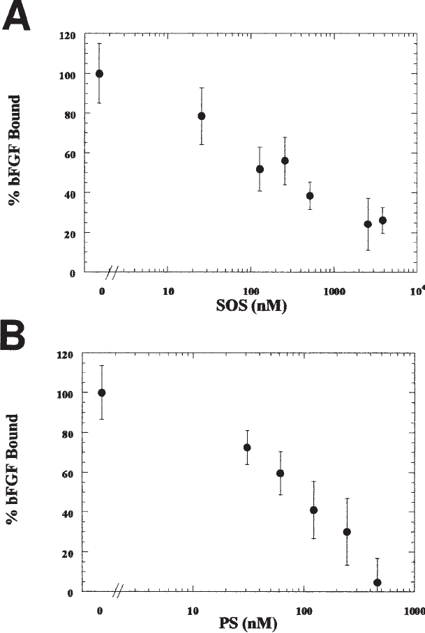
Fig. 2. Inhibitors of bFGF-E-HS Binding. E-HS (200 ng/mL), bFGF (0.056 nM), and inhibi-

tor ([A] sucrose octasulfate or SOS [B] protamine sulfate or PS) were incubated for 1 h and

then filtered across the cationic membrane. bFGF retention following incubation with SOS or

PS in the absence of E-HS was subtracted from total binding as nonspecific binding. 100%

bFGF bound corresponds to specific bFGF retention following incubation with E-HS in the

absence of inhibitor. The average ± standard error of at least triplicate samples is shown.

420 Forsten and Nugent

3.2 Analysis

3.2.1. Ligand–Proteoglycan Binding

1. The output data will represent the amount of bFGF retained on the filter for a given added

concentration. The amount retained in the absence of E-HS should be subtracted from

that with E-HS to generate data that represent specific E–HS bound bFGF.

2. Varying the concentrations of bFGF while holding constant the concentration of E-HS

(with no inhibitor), this data set should be analyzed to determine the binding capacity

(amount of bFGF bound per unit of E-HS) and the binding affinity (K

), assuming a

simple monovalent binding reaction,

which, at steady state assuming negligible ligand depletion, is described by

where R

is the binding capacity, and L

is the concentration of FGF added. The

programming to determine K

and R

is outlined below.

3. Mathematica software (Version 3.0, Wolfram Research) is launched, and a new notebook

page is initialized. Commands as outlined below are entered into the notebook page, and

the “shift” and “enter” keys are pressed simultaneously at the end of each instructional set

(symbolized in the procedure by “ ♦ ”)

4. The statistical package must be loaded by typing (see Note 2):

<<Statistics`NonlinearFit` ♦

5. Enter the volume of test solution (in liters) and the molecular weight of the growth factor

(bFGF) being investigated:

volume = 0.0002; ♦

mwF = 18000; ♦

6. Enter the amount of bFGF added per test well (L

) 〈ng〉

Fadd = {0.05, 0.05, 0.05, 0.05, 0.05, 0.05, 0.10, 0.10, 0.10, 0.10, 0.10, 0.10, 0.20, 0.20, 0.20,

0.20, 0.20, 0.20, 0.20, 0.20, 0.20, 0.20, 0.20, 0.20, 0.50, 0.50, 0.50, 0.50, 0.50, 0.50, 0.50, 0.50,

0.50, 0.75, 0.75, 0.75, 1.0, 1.0, 1.0, 1.0, 1.0, 1.0, 1.0, 1.0, 1.0, 2.0, 2.0, 2.0, 2.0, 2.0, 2.0, 2.0,

2.0, 2.0, 2.5, 2.5, 2.5, 4.0, 4.0, 4.0, 5.0, 5.0, 5.0, 5.0, 5.0, 5.0, 6.0, 6.0, 6.0, 10.0, 10.0}; ♦

7. Enter the measured values of bFGF retained (C

) 〈ng〉

Fbound = {.0025, .0035, .0034, .0013, .0055, .0033, .0067, .0069, .0076, .0028, .0033, .0035,

.017, .020, .018, .0063, .0076, .0063, .017, .016, .018, .016, .017, .017, .079, .034, .043, .029,

.034, .032, .021, .022, .020, .047, .056, .057, .080, .13, .099, .13, .071, .078, .037, .039, .086,

.088, .066, .070, .21, .24, .19, .17, .16, .16, .25, .20, .22, .32, .32, .30, .17, .37, .27, .22, .20, .17,

.51, .48, .45, .44, .39, .42}; ♦

8. Convert these values (L

and C

) from ng to nM and store as data sets 1 and 2:

dat1 = Fadd/(volume*mwF) ; ♦

dat2 = Fbound/(volume*mwF); ♦

+ L

P + L

Growth Factor Binding 421

9. Group the data (L

, C

data = {dat1, dat2}; ♦

binding = Transpose[data]; ♦

10. Perform the calculation for the nonlinear regression—ParameterCITable will output the

and R

values at the end with the standard error and the confidence interval. The units

for each will be in nM:

ParameterCITable /. NonlinearRegress[binding, ligand*Rt/(Kd1+ligand),

{ligand}, {Rt,Kd1}] ♦

11. K

is 2.3 ± 0.6 nM. R

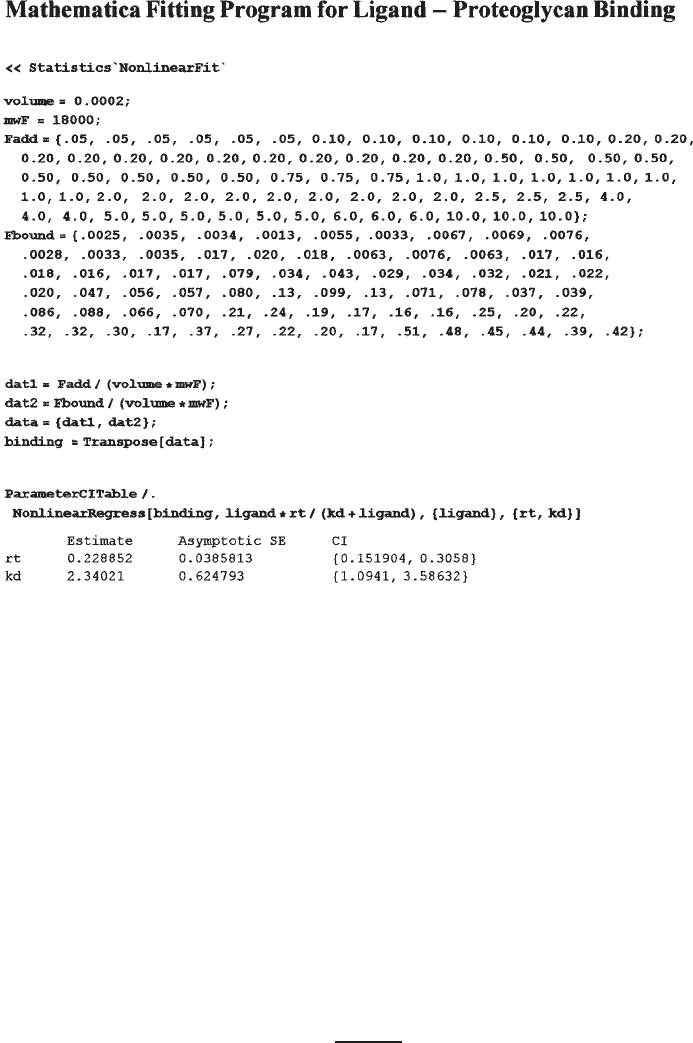
is 0.23 ± 0.04 nM. The complete Mathematica program is shown

in Fig. 3. To convert R

to sites/ng E-HS (see Note 3):

Fig. 3. Mathematica program to solve for ligand–proteoglycan affinity and binding sites.

The code and data are input as shown. The ; following each line suppresses output and may be

eliminated if the user prefers. The output is displayed at the bottom and includes the asymptotic

standard error and the asymptotic confidence intervals.

sites = R

volume

422 Forsten and Nugent

where PG is the amount of E-HS added 〈ng〉, N

is Avogadro’s number <6.02 * 10

sites mol>. R

for this system is 7.0 ± 1.2 × 10

sites/ng.

Although similar, the specifics for the ligand-binding inhibitor and the proteoglycan bind-

ing inhibitor do differ slightly and will each be outlined below. As example inhibitors, we

include data for sucrose octasulfate (ligand-binding inhibitor) and protamine sulfate

(proteoglycan-binding inhibitor)

3.2.2. Ligand-Binding Inhibitors (Sodium Sucrose Octasulfate)

An analysis of the inhibitor effectiveness is conducted based on steady-state data

acquisition with two independent first-order reactions occurring in solution.

(1)

(2)

where P is E-HS, L is the growth factor (bFGF), C

is the binding complex of E-HS

and bFGF, S is a growth factor binding inhibitor (SOS), and C

is the binding complex

of SOS and bFGF.

Assuming conservation of mass, the following equation at the steady state can be

solved for the K

value (K

– C

)(L

– C

)– (P

– C

= K

(4)

where

Knowing P

and K

from steady-state analysis in the absence of inhibitor (see

Subheading 3.2.), experiments are run at a constant level of E-HS and bFGF (L

) and

various levels of inhibitor (S

). Retention is a measurement of C

. The programming

to determine K

is outlined below.

1. Mathematica software (Version 3.0, Wolfram Research) is launched, and a new notebook

page is initialized. Commands as outlined below are entered into the notebook page, and

the “shift” and “enter” key are pressed simultaneously at the end of each instructional set

(symbolized in the procedure by “ ♦ ”)

2. The statistical package must be loaded by typing (see Note 2)

<<Statistics`NonlinearFit` ♦

3. The known parameters—P

and K

—with both in units of nM:

= 0.23; ♦

= 2.3; ♦

4. Enter the ligand concentration, L

〈nM〉, the reaction volume, volume 〈L〉, the molecular

weight of the inhibitor, mwI 〈g/mol〉, and the molecular weight of the growth factor,

mwF 〈g/mol〉:

= 0.056; ♦

volume = 0.0002; ♦

mwI = 1159; ♦

mwF = 18000; ♦

– C

+ S

+ K

– L

– C

+ S

+ K

–4S

– C

P + L

S + L

Growth Factor Binding 423

5. Enter the quantity of inhibitor (S

) added 〈ng〉:

s = {0, 0, 0, 0, 5, 5, 5, 25, 25, 25, 50, 50, 50, 100, 100, 100, 500, 500, 500, 750, 750, 750}; ♦

6. Enter the measured values of bFGF retained (C

) 〈ng〉:

c = {.018, .015, .022, .021, .02, .016, .013, .011, .0061, .011, .0082, .0061,

.013, .0094, .010, .0076, .0072, .0015, .0052, .0073, .0040, .0039}; ♦

7. Convert these values (S

and C

) to nM from ng and store as data sets A and B:

dat1 = s/(volume*mwI) ; ♦

dat2 = c/(volume*mwF); ♦

8. Enter K

as a set of data:

dat3 = Kd1*dat2; ♦

9. Group the data (S

, C

, K

data = {dat1, dat2, dat3}; ♦

SOS = Transpose[data]; ♦

10. Perform the calculation for the nonlinear regression—ParameterCITable will output the

value at the end, with the standard error and the confidence interval. Entering an

estimate or initial guess for K

will aid in the fitting process (the initial guess in our

example was 300; see Note 4). It should be noted that the C

value corresponds to one of

the roots of the quadratic equation (note the minus sign shown bold below)—the alternate

root yielded a negative value for K

for this case.

ParameterCITable /. NonlinearRegress[SOS, (Po-C1)*(Lo-C1)-(Po-C1)*((Lo-C1+So+Kd2) –

((Lo-C1+So+Kd2)^2-4*So*(Lo-C1))^0.5)*0.5, {So,C1}, {Kd2,300}] ♦

11. K

for SOS was 0.25 ± 0.08 µM.

3.2.3. Proteoglycan Binding Inhibitors (Protamine Sulfate)

Inhibitor effectiveness analysis is based on steady-state data acquisition with two

independent first-order reactions occurring in solution.

(1)

(2)

where P is E-HS, L is the growth factor (bFGF), C

is the binding complex of E-HS

and bFGF, PS is a proteoglycan binding inhibitor (protamine sulfate), and C

is the

binding complex of PS and bFGF.

Assuming conservation of mass, the following equation at the steady state can be

solved for the K

value (K

– C

)(P

– C

)– (L

–C

) C

= K

(3)

where

– C

+ PS

+ K

– P

– C

+ PS

+ K

– 4PS

– C

PS + L

P + L

424 Forsten and Nugent

Knowing P

and K

from steady-state analysis in the absence of inhibitor (see

Subheading 3.2.1.), experiments are run at a constant level of E-HS and bFGF (L

)

and various levels of inhibitor (PS

). Retention is a measurement of C

1. Mathematica software (Version 3.0, Wolfram Research) is launched, and a new notebook

page is initialized. Commands as outlined below are entered into the notebook page, and

the “shift” and “enter” keys are pressed simultaneously at the end of each instructional set

(symbolized in the procedure by “ ♦ ”)

2. The statistical package must be loaded by typing (see Note 2):

<<Statistics`NonlinearFit` ♦

3. The known parameters are then initialized—P

and K

—with both in units of nM:

= 0.23; ♦

= 2.3; ♦

4. Enter the ligand concentration - L

〈nM〉, the reaction volume, volume 〈L〉, the molecular

weight of the inhibitor - mwI 〈g/mol〉, and the molecular weight of the growth factor - mwF

〈g/mol〉:

= 0.056; ♦

volume = 0.0002; ♦

mwI = 6500; ♦

mwF = 18000; ♦

5. Enter the quantity of inhibitor (S

) added 〈ng〉:

s = {0, 0, 0, 40, 40, 40, 80, 80, 80, 160, 160, 160, 320, 320, 320, 600, 600, 600}; ♦

6. Enter the measured values of bFGF retained (C

) 〈ng〉:

c = {.018, .022, .019, .014, .017, .014, .009, .013, .014, .01, .012, .003, .001, .006, .011,

.003, .002, -.003}; ♦

7. Convert these values (PS

and C

) from ng to nM and store as data sets A and B:

dat1 = s/(volume*mwI) ; ♦

dat2 = c/(volume*mwF); ♦

8. Enter K

as a set of data:

dat3 = Kd1*dat2; ♦

9. Group the data (PS

, C

, K

data = {dat1, dat2, dat3}; ♦

Protamine = Transpose[data]; ♦

10. Perform the calculation for the nonlinear regression—ParameterCITable will output the

value at the end or with the standard error and the confidence interval. Entering an

estimate or initial guess for K

will aid in the fitting process (the initial guess in our

example was 75) (see Note 4). It should be noted that the C

value corresponds to one of

Growth Factor Binding 425

the roots of the quadratic equation (note the minus sign shown bold below)—the alternate

root yielded a negative value for K

for this case.

ParameterCITable /. NonlinearRegress[Protamine, (L

– C

)*(P

– C

)– (L

- C

)

((P

–

+ PS + K

) – ((P

– C

+ PS + K

) ^ 2 – 4

- C

)) ^ 0.5)

0.5, {PS,C

,75}] ♦

10. K

for protamine sulfate was 0.1 ± 0.02 µM.

3.3. Summary

Proteoglycan binding is a physiologically important means of regulating growth

factor activity and availability. This chapter details a fast and simple assay for

quantifying inhibitors of growth factor–proteoglycan binding. Although data and

the corresponding analysis focused on inhibitors of bFGF interactions, the method

should be easily transferable to other proteoglycan-binding growth factors and

molecules.

4. Notes

1. Many protocols for isolation of proteoglycans involve the use of denaturing agents such

as urea. These agents can interfere with protein–proteoglycan interactions and should be

removed from proteoglycan preparation prior to binding experiments.

2. When loading the Statistics packages, it is important to use ` (grave accent) as opposed to

‘ (open quote) in the statement: <<Statistics`NonlinearFit`.

3. In calculating the growth-factor binding sites per nanogram of proteoglycan, it is impor-

tant to enter the R

value in moles per liter, volume in liters, and proteoglycan in nano-

gram to generate binding sites per nanogram (see Subheading 3.2.1, step 11).

4. When fitting parameters using NonlinearRegress, a warning may be issued:

NonlinearFit::lmpnocon : Warning: The sum of squares has achieved a

minimum, but at least one parameter estimate fails to satisfy either an accuracy

goal of 1 digit (S) or a precision goal of 1 digit (s). These goals are less

strict than those for the sum of squares, specified by AccuracyGoal ->6 and

PrecisionGoal ->

If this occurs, it is best to rerun your regression fit with the output K

used as your new

initial guess. This may be easily done by highlighting the right sidebar and pressing ♦.

Repeat this procedure until the warning is not issued.

References

1. Conrad, E. (1998) Heparin Binding Proteins, Academic Press, San Diego, CA.

2. Rapraeger, A. C., Krufka, A., and Olwin, B. B. (1991) Requirement of heparan sulfate for

bFGF-mediated fibroblast growth and myoblast differentiation. Science 252, 1705–1708.

3. Fannon, M. and Nugent, M. A. (1996) Basic fibroblast growth factor binds its receptors, is

internalized, and stimulates DNA sythesis in Balb/c3T3 cells in the absence of heparan

sulfate. J. Biol. Chem. 271, 17949–17956.

4. Forsten, K. E., Courant, N. A., and Nugent, M. A. (1997) Endothelial proteoglycans inhibit

bFGF binding and mitogenesis. J. Cell. Physiol. 172, 209–220.

5. Dowd, C. J., Cooney, C. L., and Nugent, M. A. (1999) Heparan sulfate mediates bFGF

transport through basement membrane by diffusion with rapid reversible binding. J. Biol.

Chem. 274, 5236–5244.

426 Forsten and Nugent

6. Isner, J. M. (1996) The role of angiogenic cytokines in cardiovascular disease. Clin.

Immunol. Immunopathol. 80, S82–S91.

7. Rapraeger, A. and Yeaman, C. (1989) A quantitative solid-phase assay for identifying

radiolabeled glycosaminoglycans in crude cell extracts. Anal. Biochem. 179, 361–365.

8. Nugent, M. A. and Edelman, E. R. (1992) Kinetics of basic fibroblast growth factor bind-

ing to its receptor and heparan sulfate proteoglycan: a mechanism for cooperativity. Bio-

chemistry 31, 8876–8883.

9. Farndale, R. W., Buttle, D. J., and Barrett, A. J. (1986) Improved quantitation and dis-

crimination of sulphated glycosaminoglycans by use of dimethylmethylene blue. Biochim.

Biophys. Acta 883, 173–177.

Interaction with RTKs 427

427

From:

Methods in Molecular Biology, Vol. 171: Proteoglycan Protocols

Interaction of Proteoglycans

with Receptor Tyrosine Kinases

David K. Moscatello and Renato V. Iozzo

1. Introduction

The control of cell proliferation depends on the interactions between growth factors

and their specific receptor-activated signaling pathways. It is well accepted that the

local extracellular matrix can modulate cellular responses to a given signal in several

ways, such as by modulating the affinity of the ligand for its cognate receptor (1), by

binding and limiting availability of a growth factor (1–3), or by influencing proteolytic

processing and internalization (3). However, it has only recently been shown that

“structural” components of the extracellular matrix can interact directly with, and

activate, receptor tyrosine kinases (RTKs). This was first shown by Vogel et al. and

Shrivastava et al., who demonstrated that the “orphan” receptor tyrosine kinases DDR1

and DDR2 in fact bind fibrillar collagen (4,5). This binding required the native triple-

helical structure of collagen and showed much slower kinetics than observed with

other ligand–receptor interactions (5). Decorin (6–8), a member of a family of small

leucine-rich proteoglycans (3), binds to fibrillar collagen and is an important regulator

of matrix assembly (9–11). Decorin content is elevated in the tumor stroma of colon

cancer (11), and ectopic expression of decorin inhibits cell growth (11–13). The

growth-suppressive properties of decorin are independent of p53 or retinoblastoma

proteins but require functional p21 protein (Waf1/Cip1/Sdi1) (13–16).

We recently reported that decorin activated the epidermal growth factor receptor

(EGFR) in A431 squamous carcinoma cells and other transformed cell lines. This

signaling was mediated by the protein core of decorin and induced MAP kinase

activation and a protracted upregulation of endogenous p21, thereby leading to growth

suppression (17). This activation occurred as a result of a direct interaction of decorin

with the EGF receptor (17,18). However, even “small” proteoglycans such as decorin

(~100 kDa, with a ~42-kDa core protein) are quite large in comparison with most

ligands of receptor tyrosine kinases, which are typically 6–25 kDa, a fact that compli-

cates analysis of crosslinking studies. Thus, in combination with their relatively