Hirsch M.J., Pardalos P.M., Murphey R. Dynamics of Information Systems: Theory and Applications
Подождите немного. Документ загружается.

66 K.D. Pham
−Tr
Y
i,1
20
(s)Π
i
02
(s) +Y
i,1
21
(s)Π
i
12
(s) +Y
i,1
22
(s)Π
i
22
(s)
−p
T
i
(s)R
i
(s)p
i
(s) −p
T
zi
(s)R
zi
(s)p
zi
(s)
G
i,r
s,Y
i
00
,Y
i
01
,Y
i
02
,Y
i
10
,Y
i
11
,Y
i
12
,Y
i
20
,Y
i
21
,Y
i
22
,
˘
Z
i
0
,
˘
Z
i
2
;p
i
,p
zi
=−2
˘
Z
i,r
0
T
(s)
B
i
(s)p
i
(s) +C
i
(s)p
zi
(s) +E
i
(s)d
i
(s)
−2
˘
Z
i,r
2
T
(s)E
zi
(s)d
mi
(s)
−Tr
Y
i,r
00
(s)Π
i
00
(s) +Y
i,r
01
(s)Π
i
10
(s) +Y
i,r
02
(s)Π
i
20
(s)
−Tr
Y
i,r
10
(s)Π
i
01
(s) +Y
i,r
11
(s)Π
i
11
(s) +Y
i,r
12
(s)Π
i
21
(s)
−Tr
Y
i,r
20
(s)Π
i
02
(s) +Y
i,r
21
(s)Π
i
12
(s) +Y
i,r
22
(s)Π
i
22
(s)
provided that all the k
i
-tuple variables are given by
Y
i
00
(·)
Y
i,1
00
(·),...,Y
i,k
i
00
(·)
≡
H
i
00
(·, 1),...,H
i
00
(·,k
i
)
Y
i
01
(·)
Y
i,1
01
(·),...,Y
i,k
i
01
(·)
≡
H
i
01
(·, 1),...,H
i
01
(·,k
i
)
Y
i
02
(·)
Y
i,1
02
(·),...,Y
i,k
i
02
(·)
≡
H
i
02
(·, 1),...,H
i
02
(·,k
i
)
Y
i
10
(·)
Y
i,1
10
(·),...,Y
i,k
i
10
(·)
≡
H
i
10
(·, 1),...,H
i
10
(·,k
i
)
Y
i
11
(·)
Y
i,1
11
(·),...,Y
i,k
i
11
(·)
≡
H
i
11
(·, 1),...,H
i
11
(·,k
i
)
Y
i
12
(·)
Y
i,1
12
(·),...,Y
i,k
i
12
(·)
≡
H
i
12
(·, 1),...,H
i
12
(·,k
i
)
Y
i
20
(·)
Y
i,1
20
(·),...,Y
i,k
i
20
(·)
≡
H
i
20
(·, 1),...,H
i
20
(·,k
i
)
Y
i
21
(·)
Y
i,1
21
(·),...,Y
i,k
i
21
(·)
≡
H
i
21
(·, 1),...,H
i
21
(·,k
i
)
Y
i
22
(·)
Y
i,1
22
(·),...,Y
i,k
i
22
(·)
≡
H
i
22
(·, 1),...,H
i
22
(·,k
i
)
˘
Z
i
0
(·)
˘
Z
i,1
0
(·),...,
˘
Z
i,k
i
0
(·)
≡
˘
D
i
0
(·, 1),...,
˘
D
i
0
(·,k
i
)
˘
Z
i
1
(·)
˘
Z
i,1
1
(·),...,
˘
Z
i,k
i
1
(·)
≡
˘
D
i
1
(·, 1),...,
˘
D
i
1
(·,k
i
)
˘
Z
i
2
(·)
˘
Z
i,1
2
(·),...,
˘
Z
i,k
i
2
(·)
≡
˘
D
i
2
(·, 1),...,
˘
D
i
2
(·,k
i
)
Z
i
0
(·)
Z
i,1
0
(·),...,Z
i,k
i
0
(·)
≡
D
i
0
(·, 1),...,D
i
0
(·,k
i
)
Now it is straightforward to establish the product mappings
F
i
00
F
i,1
00
×···×F
i,k
i
00
F
i
01
F
i,1
01
×···×F
i,k
i
01
F
i
02
F
i,1
02
×···×F
i,k
i
02
F
i
10
F
i,1
10
×···×F
i,k
i
10
F
i
11
F
i,1
11
×···×F
i,k
i
11
F
i
12
F
i,1
12
×···×F
i,k
i
12

3 Performance-Information Analysis and Distributed Feedback Stabilization 67
F
i
20
F
i,1
20
×···×F
i,k
i
20
F
i
21
F
i,1
21
×···×F
i,k
i
21
F
i
22
F
i,1
22
×···×F
i,k
i
22
˘
G
i
0
˘
G
i,1
0
×···×
˘
G
i,k
i
0
˘
G
i
1
˘
G
i,1
1
×···×
˘
G
i,k
i
1
˘
G
i
2
˘
G
i,1
2
×···×
˘
G
i,k
i
2
G
i
G
i,1
×···×G
i,k
i
Thus, the dynamic equations (3.32)–(3.57) can be rewritten compactly as follows
d
ds
Y
i
00
(s) =F
i
00
s,Y
i
00
(s), Y
i
01
(s), Y
i
20
(s);K
i
(s), K
zi
(s)
,Y
i
00
(t
f
) (3.58)
d
ds
Y
i
01
(s) =F
i
01
s,Y
i
00
(s), Y
i
01
,Y
i
11
(s), Y
i
21
(s);K
i
(s), K
zi
(s)
,Y
i
01
(t
f
) (3.59)
d
ds
Y
i
02
(s) =F
i
02
s,Y
i
02
,Y
i
12
(s), Y
i
22
(s);K
i
(s), K
zi
(s)
,Y
i
02
(t
f
) (3.60)
d
ds
Y
i
10
(s) =F
i
10
s,Y
i
00
(s), Y
i
10
(s), Y
i
20
(s);K
i
(s), K
zi
(s)
,Y
i
10
(t
f
) (3.61)
d
ds
Y
i
11
(s) =F
i
11
s,Y
i
01
(s), Y
i
10
(s), Y
i
11
(s), Y
i
21
(s)
,Y
i
11
(t
f
) (3.62)
d
ds
Y
i
12
(s) =F
i
12
s,Y
i
02
(s), Y
i
12
(s), Y
i
22
(s)
,Y
i
12
(t
f
) (3.63)
d
ds
Y
i
20
(s) =F
i
20
s,Y
i
00
(s), Y
i
10
(s), Y
i
20
(s);K
i
(s), K
zi
(s)
,Y
i
20
(t
f
) (3.64)
d
ds
Y
i
21
(s) =F
i
21
s,Y
i
01
(s), Y
i
11
(s), Y
i
20
(s), Y
i
21
(s)
,Y
i
21
(t
f
) (3.65)
d
ds
Y
i
22
(s) =F
i
22
s,Y
i
02
(s), Y
i
12
(s), Y
i
22
(s)
,Y
i
22
(t
f
) (3.66)
d
ds
˘
Z
i
0
(s) =
˘
G
i
0
s,Y
i
00
(s), Y
i
02
(s),
˘
Z
i
0
(s);K
i
(s), K
zi
(s);p
i
(s), p
zi
(s)
,
˘
Z
i
0
(t
f
) (3.67)
d
ds
˘
Z
i
1
(s) =
˘
G
i
1
s,Y
i
10
(s), Y
i
12
(s),
˘
Z
i
0
(s),
˘
Z
i
1
(s);p
i
(s), p
zi
(s)
,
˘
Z
i
1
(t
f
) (3.68)
d
ds
˘
Z
i
2
(s) =
˘
G
i
2
s,Y
i
20
,Y
i
22
(s),
˘
Z
i
2
(s);p
i
(s), p
zi
(s)
,
˘
Z
i
2
(t
f
) (3.69)
d
ds
Z
i
(s) =G
i
s,Y
i
00
(s), Y
i
01
(s), Y
i
02
(s), Y
i
10
(s), Y
i
11
(s), Y
i
12
(s), Y
i
20
(s), . . .
Y
i
21
(s), Y
i
22
(s),
˘
Z
i
0
(s),
˘
Z
i
2
(s);p
i
(s), p
zi
(s)
,Z
i
(t
f
) (3.70)
where the terminal-value conditions are defined by
Y
i
00
(t
f
) Q
f
i
×0 ×···×0 Y
i
01
(t
f
) Q
f
i
×0 ×···×0
68 K.D. Pham
Y
i
02
(t
f
) 0 ×0 ×···×0 Y
i
10
(t
f
) Q
f
i
×0 ×···×0
Y
i
11
(t
f
) Q
f
i
×0 ×···×0 Y
i
12
(t
f
) 0 ×0 ×···×0
Y
i
20
(t
f
) 0 ×0 ×···×0 Y
i
21
(t
f
) 0 ×0 ×···×0
Y
i
22
(t
f
) 0 ×0 ×···×0
˘
Z
i
0
(t
f
) 0 ×0 ×···×0
˘
Z
i
1
(t
f
) 0 ×0 ×···×0
˘
Z
i
2
(t
f
) 0 ×0 ×···×0
Z
i
(t
f
) 0 ×0 ×···×0
Note that for each agent i the product system (3.58)–(3.70) uniquely determines
Y
i
00
, Y
i
01
, Y
i
02
, Y
i
10
, Y
i
11
, Y
i
12
, Y
i
20
, Y
i
21
, Y
i
22
,
˘
Z
i
0
,
˘
Z
i
1
,
˘
Z
i
2
, and Z
i
once the admissible
4-tuple (K
i
,K
zi
,p
i
,p
zi
) is specified. Thus, Y
i
00
, Y
i
01
, Y
i
02
, Y
i
10
, Y
i
11
, Y
i
12
, Y
i
20
, Y
i
21
,
Y
i
22
,
˘
Z
i
0
,
˘
Z
i
1
,
˘
Z
i
2
, and Z
i
are considered as the functions of K
i
, K
zi
, p
i
, and p
zi
.
The performance index for the interconnected system can therefore be formulated
in terms of K
i
, K
zi
, p
i
, and p
zi
for agent i.
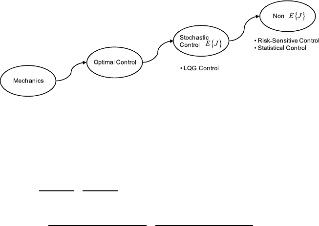
The subject of risk taking has been of great interest not only to control system de-
signers of engineered systems but also to decision makers of financial systems. One
approach to study risk in stochastic control system is exemplified in the ubiquitous
theory of linear-quadratic Gaussian (LQG) control whose preference of expected
value of performance measure associated with a class of stochastic systems is min-
imized against all random realizations of the uncertain environment. Other aspects
of performance distributions that do not appear in the classical theory of LQG are
variance, skewness, kurtosis, etc. For instance, it may nevertheless be true that some
performance with negative skewness appears riskier than performance with positive
skewness when expectation and variance are held constant. If skewness does, in-
deed, play an essential role in determining the perception of risk, then the range of
applicability of the present theory should be restricted, for example, to symmetric
or equally skewed performance measures.
There have been several studies that attempt to generalize the present LQG the-
ory to account for the effects of variance [11] and [6] or of other description of
probability density [12] on the perceived riskiness of performance measures. The
contribution of this research is to directly address the perception of risk via a selec-
tive set of performance distribution characteristics of its outcomes governed by ei-
ther dispersion, skewness, flatness, etc. or a combination thereof. Figure 3.4 depicts
some possible interpretations on measures of performance risk for control decision
under uncertainty.
Definition 1 (Risk-value aware performance index) Associate with agent i the
k
i
∈Z
+
and the sequence μ
i
={μ
i
r
≥0}
k
i
r=1
with μ
i
1
> 0. Then, for (t
0
,x
0
i
) given,
the risk-value aware performance index
φ
i
0
:{t
0
}×
R
n
i
×n
i
k
i
×
R
n
i
k
i
×R
k
i
→R
+
over a finite optimization horizon is defined by a risk-value model to reflect the
tradeoff between value and riskiness of the Chi-squared type performance mea-
3 Performance-Information Analysis and Distributed Feedback Stabilization 69
Fig. 3.4 Measures of performance risk for control decision under uncertainty
sure (3.31)
φ
i
0
t
0
,Y
i
00
(·,K
i
,K
zi
,p
i
,p
zi
),
˘
Z
i
0
(·,K
i
,K
zi
,p
i
,p
zi
), Z
i
(·,K
i
,K
zi
,p
i
,p
zi
)
μ
i
1
κ
i
1
(K
i
,K
zi
,p
i
,p
zi
)
Value Measure
+μ
i
2
κ
i
2
(K
i
,K
zi
,p
i
,p
zi
) +···+μ
i
k
i
κ
i
k
i
(K
i
,K
zi
,p
i
,p
zi
)
Risk Measure
=μ
i
1
x
0
i
T
Y
i,1
00
(t
0
,K
i
,K
zi
,p
i
,p
zi
)x
0
i
+2
x
0
i
T
˘
Z
i,1
0
(t
0
,K
i
,K
zi
,p
i
,p
zi
)
+Z
i,1
0
(t
0
,K
i
,K
zi
,p
i
,p
zi
)
+μ
i
2
x
0
i
T
Y
i,2
00
(t
0
,K
i
,K
zi
,p
i
,p
zi
)x
0
i
+2
x
0
i
T
˘
Z
i,2
0
(t
0
,K
i
,K
zi
,p
i
,p
zi
) +Z
i,2
0
(t
0
,K
i
,K
zi
,p
i
,p
zi
)
+···+μ
i
k
i
x
0
i
T
Y
i,k
i
00
(t
0
,K
i
,K
zi
,p
i
,p
zi
)x
0
i
+2
x
0
i
T
˘
Z
i,k
i
0
(t
0
,K
i
,K
zi
,p
i
,p
zi
) +Z
i,k
i
0
(t
0
,K
i
,K
zi
,p
i
,p
zi
)
(3.71)
where all the parametric design measures μ
i
r
considered here by agent i, repre-
sent for different emphases on higher-order statistics and agent prioritization toward
performance robustness. Solutions {Y
i,r
00
(s, K
i
,K
zi
,p
i
,p
zi
)}
k
i
r=1
, {
˘
Z
i,r
0
(s, K
i
,K
zi
,
p
i
,p
zi
)}
k
i
r=1
and {Z
i,r
(s, K
i
,K
zi
,p
i
,p
zi
)}
k
i
r=1
when evaluated at s =t
0
satisfy the
time-backward differential equations (3.32)–(3.57) together with the terminal-value
conditions as aforementioned.
From the above definition, the statistical problem is shown to be an initial cost
problem, in contrast with the more traditional terminal cost class of investigations.
One may address an initial cost problem by introducing changes of variables which
convert it to a terminal cost problem. However, this modifies the natural context
of statistical control, which it is preferable to retain. Instead, one may take a more
direct dynamic programming approach to the initial cost problem. Such an approach
is illustrative of the more general concept of the principle of optimality, an idea
tracing its roots back to the 17th century and depicted in Fig. 3.5.
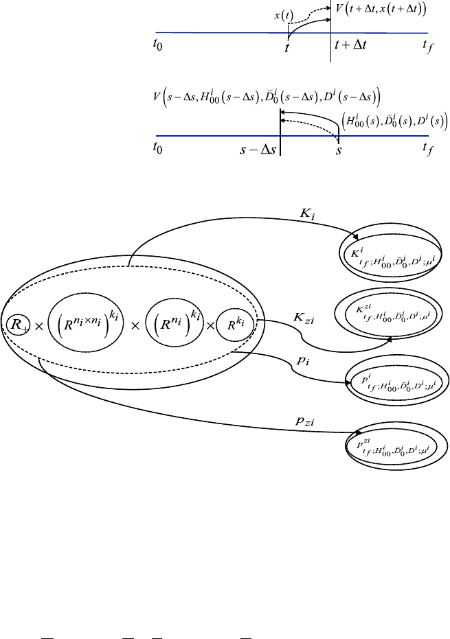
70 K.D. Pham
Fig. 3.5 Value functions in
the terminal cost problem
(top) and the initial cost
problem (bottom)
Fig. 3.6 Admissible feedback gains and interaction recovery inputs
For the given (t
f
,Y
i
00
(t
f
),
˘
Z
i
0
(t
f
), Z
i
(t
f
)), classes of K
i
t
f
,Y
i
00
(t
f
),
˘
Z
i
0
(t
f
),Z
i
(t
f
);μ
i
,
K
zi
t
f
,Y
i
00
(t
f
),
˘
Z
i
0
(t
f
),Z
i
(t
f
);μ
i
, P
i
t
f
,Y
i
00
(t
f
),
˘
Z
i
0
(t
f
),Z
i
(t
f
);μ
i
and P
zi
t
f
,Y
i
00
(t
f
),
˘
Z
i
0
(t
f
),Z
i
(t
f
);μ
i
of
admissible 4-tuple (K
i
,K
zi
,p
i
,p
zi
) are then defined.
Definition 2 (Admissible feedback gains and affine inputs) For agent i, the compact
subsets
K
i
⊂ R
n
i
×n
i
, K
zi
, P
i
⊂ R
m
i
, and P
zi
⊂ R
m
zi
be denoted by the sets of
allowable matrices and vectors as in Fig. 3.6.
Then, for k
i
∈ Z
+
, μ
i
={μ
i
r
≥ 0}
k
i
r=1
with μ
i
1
> 0, the matrix-valued sets
of K
i
t
f
,Y
i
00
(t
f
),
˘
Z
i
0
(t
f
),Z
i
(t
f
);μ
i
∈ C(t
0
,t
f
;R
m
i
×n
i
) and K
zi
t
f
,Y
i
00
(t
f
),
˘
Z
i
0
(t
f
),Z
i
(t
f
);μ
i
∈
C(t
0
,t
f
;R
m
zi
×n
i
) and the vector-valued sets of P
i
t
f
,Y
i
00
(t
f
),
˘
Z
i
0
(t
f
),Z
i
(t
f
);μ
i
∈C(t
0
,t
f
;

3 Performance-Information Analysis and Distributed Feedback Stabilization 71
R
m
i
) and P
zi
t
f
,Y
i
00
(t
f
),
˘
Z
i
0
(t
f
),Z
i
(t
f
);μ
i
∈C(t
0
,t
f
;R
m
zi
) with respective values K
i
(·) ∈
K
i
, K
zi
(·) ∈ K
zi
, p
i
(·) ∈ P
i
, and p
zi
(·) ∈ P
zi
are admissible if the resulting so-
lutions to the time-backward differential equations (3.32)–(3.57) exist on the finite
horizon [t
0
,t
f
].
The optimization problem for agent i, where instantiations are aimed at reducing
performance robustness and constituent strategies are robust to uncertain environ-
ment’s stochastic variations, is subsequently stated.
Definition 3 (Optimization of Mayer problem) Suppose that k
i
∈ Z
+
and the se-
quence μ
i
={μ
i
r
≥ 0}
k
i
r=1
with μ
i
1
> 0 are fixed. Then, the optimization prob-
lem over [t
0
,t
f
] is given by the minimization of agent i’s performance index
(3.71) over all K
i
(·) ∈ K
i
t
f
,Y
i
00
(t
f
),
˘
Z
i
0
(t
f
),Z
i
(t
f
);μ
i
, K
zi
(·) ∈ K
zi
t
f
,Y
i
00
(t
f
),
˘
Z
i
0
(t
f
),Z
i
(t
f
);μ
i
,
p
i
(·) ∈P
i
t
f
,Y
i
00
(t
f
),
˘
Z
i
0
(t
f
),Z
i
(t
f
);μ
i
and p
zi
(·) ∈P
zi
t
f
,Y
i
00
(t
f
),
˘
Z
i
0
(t
f
),Z
i
(t
f
);μ
i
subject to the
time-backward dynamical constraints (3.58)–(3.70)fors ∈[t
0
,t
f
].
It is important to recognize that the optimization considered here is in “Mayer
form” and can be solved by applying an adaptation of the Mayer form verifi-
cation theorem of dynamic programming given in [4]. In the framework of dy-
namic programming where the subject optimization is embedded into a fam-
ily of optimization based on different starting points, there is therefore a need
to parameterize the terminal time and new states by (ε, Y
i
00
,
˘
Z
i
0
,Z
i
) rather than
(t
f
,Y
i
00
(t
f
),
˘
Z
i
0
(t
f
), Z
i
(t
f
)). Thus, the values of the corresponding optimization
problems depend on the terminal-value conditions which lead to the definition of a
value function.
Definition 4 (Value function) The value function V
i
:[t
0
,t
f
]×(R
n
i
×n
i
)
k
i
×
(R
n
i
)
k
i
× R
k
i
→ R
+
associated with the Mayer problem defined as V
i
(ε, Y
i
00
,
˘
Z
i
0
,Z
i
) is the minimization of φ
i
0
(t
0
,Y
i
00
(·,K
i
,K
zi
,p
i
,p
zi
),
˘
Z
i
0
(·,K
i
,K
zi
,p
i
,
p
zi
), Z
i
(·,K
i
,K
zi
,p
i
,p
zi
)) over all K
i
(·) ∈ K
i
t
f
,Y
i
00
(t
f
),
˘
Z
i
0
(t
f
),Z
i
(t
f
);μ
i
, K
zi
(·) ∈
K
zi
t
f
,Y
i
00
(t
f
),
˘
Z
i
0
(t
f
),Z
i
(t
f
);μ
i
, p
i
(·) ∈ P
i
t
f
,Y
i
00
(t
f
),
˘
Z
i
0
(t
f
),Z
i
(t
f
);μ
i
, and p
zi
(·) ∈
P
zi
t
f
,Y
i
00
(t
f
),
˘
Z
i
0
(t
f
),Z
i
(t
f
);μ
i
subject to some (ε, Y
i
00
,
˘
Z
i
0
,Z
i
) ∈[t
0
,t
f
]×(R
n
i
×n
i
)
k
i
×
(R
n
i
)
k
i
×R
k
i
.
It is conventional to let V
i
(ε, Y
i
00
,
˘
Z
i
0
,Z
i
) =∞when K
i
t
f
,Y
i
00
(t
f
),
˘
Z
i
0
(t
f
),Z
i
(t
f
);μ
i
,
K
zi
t
f
,Y
i
00
(t
f
),
˘
Z
i
0
(t
f
),Z
i
(t
f
);μ
i
, P
i
t
f
,Y
i
00
(t
f
),
˘
Z
i
0
(t
f
),Z
i
(t
f
);μ
i
and P
zi
t
f
,Y
i
00
(t
f
),
˘
Z
i
0
(t
f
),Z
i
(t
f
);μ
i
are
empty. To avoid cumbersome notation, the dependence of trajectory solutions on
K
i
, K
zi
, p
i
and p
zi
is now suppressed. Next, some candidates for the value function
can be constructed with the help of a reachable set.

72 K.D. Pham
Definition 5 (Reachable set) At agent i, let the reachable set Q
i
be defined as fol-
lows
Q
i
ε, Y
i
00
,
˘
Z
i
0
,Z
i
∈[t
0
,t
f
]×
R
n
i
×n
i
k
i
×
R
n
i
k
i
×R
k
i
such that
K
i
t
f
,Y
i
00
(t
f
),
˘
Z
i
0
(t
f
),Z
i
(t
f
);μ
i
×K
zi
t
f
,Y
i
00
(t
f
),
˘
Z
i
0
(t
f
),Z
i
(t
f
);μ
i
×
P
i
t
f
,Y
i
00
(t
f
),
˘
Z
i
0
(t
f
),Z
i
(t
f
);μ
i
×P
zi
t
f
,Y
i
00
(t
f
),
˘
Z
i
0
(t
f
),Z
i
(t
f
);μ
i
not empty
Moreover, it can be shown that the value function is satisfying a partial differen-
tial equation at each interior point of Q
i
at which it is differentiable.
Theorem 4 (Hamilton–Jacobi–Bellman (HJB) equation for Mayer problem) For
agent i, let (ε, Y
i
00
,
˘
Z
i
0
,Z
i
) be any interior point of the reachable set Q
i
at
which the value function V
i
(ε, Y
i
00
,
˘
Z
i
0
,Z
i
) is differentiable. If there exists an
optimal 4-tuple control strategy (K
∗
i
,K
∗
zi
,p
∗
i
,p
∗
zi
) ∈ K
i
t
f
,Y
i
00
(t
f
),
˘
Z
i
0
(t
f
),Z
i
(t
f
);μ
i
×
K
zi
t
f
,Y
i
00
(t
f
),
˘
Z
i
0
(t
f
),Z
i
(t
f
);μ
i
×P
i
t
f
,Y
i
00
(t
f
),
˘
Z
i
0
(t
f
),Z
i
(t
f
);μ
i
×P
zi
t
f
,Y
i
00
(t
f
),
˘
Z
i
0
(t
f
),Z
i
(t
f
);μ
i
, the
partial differential equation associated with agent i
0 = min
K
i
∈K
i
,K
zi
∈K
zi
,p
i
∈P
i
,p
zi
∈P
zi
∂
∂ε
V
i
ε, Y
i
00
,
˘
Z
i
0
,Z
i
+
∂
∂ vec(Y
i
00
)
V
i
ε, Y
i
00
,
˘
Z
i
0
,Z
i
·vec
F
i
00
ε;Y
i
00
,Y
i
01
,Y
i
20
;K
i
,K
zi
+
∂
∂ vec(
˘
Z
i
0
)
V
i
ε, Y
i
00
,
˘
Z
i
0
,Z
i
·vec
˘
G
i
0
ε;Y
i
00
,Y
i
02
,
˘
Z
i
0
;K
i
,K
zi
;p
i
,p
zi
+
∂
∂ vec(Z
i
)
V
i
ε, Y
i
00
,
˘
Z
i
0
,Z
i
·vec
G
i
ε;Y
i
00
,Y
i
00
,Y
i
01
,Y
i
02
,Y
i
10
,Y
i
11
,Y
i
12
,Y
i
20
,Y
i
21
,Y
i
22
,
˘
Z
i
0
,
˘
Z
i
2
;p
i
,p
zi
(3.72)
is satisfied together with V
i
(t
0
,Y
i
00
,
˘
Z
i
0
,Z
i
) = φ
i
0
(t
0
,Y
i
00
,
˘
Z
i
0
,Z
i
) and vec(·) the
vectorizing operator of enclosed entities. The optimum in (3.72) is achieved by the
4-tuple control decision strategy (K
∗
i
(ε), K
∗
zi
(ε), p
∗
i
(ε), p
∗
zi
(ε)) of the optimal deci-
sion strategy at ε.
Proof Detail discussions are in [4] and the modification of the original proofs
adapted to the framework of statistical control together with other formal analysis
can be found in [7] which is available via http://etd.nd.edu/ETD-db/theses/available/
etd-04152004-121926/unrestricted/PhamKD052004.pdf.
Finally, the next theorem gives the sufficient condition used to verify optimal
decisions for the interconnected system or agent i.

3 Performance-Information Analysis and Distributed Feedback Stabilization 73
Theorem 5 (Verification theorem) Fix k
i
∈Z
+
. Let W
i
(ε, Y
i
00
,
˘
Z
i
0
,Z
i
) be a contin-
uously differentiable solution of the HJB equation (3.72) and satisfy the boundary
condition
W
i
t
0
,Y
i
00
,
˘
Z
i
0
,Z
i
=φ
i
0
t
0
,Y
i
00
,
˘
Z
i
0
,Z
i
(3.73)
Let (t
f
,Y
i
00
(t
f
),
˘
Z
i
0
(t
f
), Z
i
(t
f
)) be a point of Q
i
;4-tuple (K
i
,K
zi
,p
i
,p
zi
) in
K
i
t
f
,Y
i
00
(t
f
),
˘
Z
i
0
(t
f
),Z
i
(t
f
);μ
i
× K
zi
t
f
,Y
i
00
(t
f
),
˘
Z
i
0
(t
f
),Z
i
(t
f
);μ
i
× P
i
t
f
,Y
i
00
(t
f
),
˘
Z
i
0
(t
f
),Z
i
(t
f
);μ
i
×
P
zi
t
f
,Y
i
00
(t
f
),
˘
Z
i
0
(t
f
),Z
i
(t
f
);μ
i
; and Y
i
00
,
˘
Z
i
0
, and Z
i
the corresponding solutions of (3.58)–
(3.70). Then, W
i
(s, Y
i
00
(s),
˘
Z
i
0
(s), Z
i
(s)) is time-backward increasing in s. If
(K
∗
i
,K
∗
zi
,p
∗
i
,p
∗
zi
) is a 4-tuple in K
i
t
f
,Y
i
00
(t
f
),
˘
Z
i
0
(t
f
),Z
i
(t
f
);μ
i
×K
zi
t
f
,Y
i
00
(t
f
),
˘
Z
i
0
(t
f
),Z
i
(t
f
);μ
i
×P
i
t
f
,Y
i
00
(t
f
),
˘
Z
i
0
(t
f
),Z
i
(t
f
);μ
i
×P
zi
t
f
,Y
i
00
(t
f
),
˘
Z
i
0
(t
f
),Z
i
(t
f
);μ
i
defined on [t
0
,t
f
] with cor-
responding solutions, Y
i∗
00
,
˘
Z
i∗
0
and Z
i∗
of the dynamical equations such that
0 =
∂
∂ε
W
i
s,Y
i∗
00
(s),
˘
Z
i∗
0
(s), Z
i∗
(s)
+
∂
∂ vec(Y
i
00
)
W
i
s,Y
i∗
00
(s),
˘
Z
i∗
0
(s), Z
i∗
(s)
·vec
F
i
00
s;Y
i∗
00
(s), Y
i∗
01
(s), Y
i∗
20
(s);K
∗
i
(s), K
∗
zi
(s)
+
∂
∂ vec(
˘
Z
i
0
)
W
i
s,Y
i∗
00
(s),
˘
Z
i∗
0
(s), Z
i∗
(s)
·vec
˘
G
i
0
s;Y
i∗
00
(s), Y
i∗
02
(s),
˘
Z
i∗
0
(s);K
∗
i
(s), K
∗
zi
(s);p
∗
i
(s), p
∗
zi
(s)
+
∂
∂ vec(Z
i
)
W
i
s,Y
i∗
00
(s),
˘
Z
i∗
0
(s), Z
i∗
(s)
·vec
G
i
ε;Y
i∗
00
(s), Y
i∗
00
(s), Y
i∗
01
(s), Y
i∗
02
(s), Y
i∗
10
(s), Y
i∗
11
(s), Y
i∗
12
(s),
Y
i∗
20
(s), Y
i∗
21
(s), Y
i∗
22
(s),
˘
Z
i∗
0
(s),
˘
Z
i∗
2
(s);p
∗
i
(s), p
∗
zi
(s)
(3.74)
then (K
∗
i
,K
∗
zi
,p
∗
i
,p
∗
zi
) in K
i
t
f
,Y
i
00
(t
f
),
˘
Z
i
0
(t
f
),Z
i
(t
f
);μ
i
× K
zi
t
f
,Y
i
00
(t
f
),
˘
Z
i
0
(t
f
),Z
i
(t
f
);μ
i
×
P
i
t
f
,Y
i
00
(t
f
),
˘
Z
i
0
(t
f
),Z
i
(t
f
);μ
i
×P
zi
t
f
,Y
i
00
(t
f
),
˘
Z
i
0
(t
f
),Z
i
(t
f
);μ
i
is optimal and
W
i
ε, Y
i
00
,
˘
Z
i
0
,Z
i
=V
i
ε, Y
i
00
,
˘
Z
i
0
,Z
i
(3.75)
where V
i
(ε, Y
i
00
,
˘
Z
i
0
,Z
i
) is the value function.
Proof Due to the length limitation, the interested reader is referred to the work by
the author [7] which can be found via http://etd.nd.edu/ETD-db/theses/available/
etd-04152004-121926/unrestricted/PhamKD052004.pdf for the detail proof and
other relevant analysis.
Note that, to have a solution (K
∗
i
,K
∗
zi
,p
∗
i
,p
∗
zi
) ∈ K
i
t
f
,Y
i
00
(t
f
),
˘
Z
i
0
(t
f
),Z
i
(t
f
);μ
i
×
K
zi
t
f
,Y
i
00
(t
f
),
˘
Z
i
0
(t
f
),Z
i
(t
f
);μ
i
×P
i
t
f
,Y
i
00
(t
f
),
˘
Z
i
0
(t
f
),Z
i
(t
f
);μ
i
×P
zi
t
f
,Y
i
00
(t
f
),
˘
Z
i
0
(t
f
),Z
i
(t
f
);μ
i
well
74 K.D. Pham
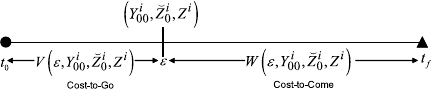
Fig. 3.7 Cost-to-go in the
sufficient condition to
Hamilton–Jacobi–Bellman
equation
defined and continuous for all s ∈[t
0
,t
f
], the trajectory solutions Y
i
00
(s),
˘
Z
i
0
(s)
and Z
i
(s) to the dynamical equations (3.58)–(3.70) when evaluated at s = t
0
must
then exist. Therefore, it is necessary that Y
i
00
(s),
˘
Z
i
0
(s) and Z
i
(s) are finite for all
s ∈[t
0
,t
f
). Moreover, the solutions of the dynamical equations (3.58)–(3.70)ex-
ist and are continuously differentiable in a neighborhood of t
f
. Applying the results
from [2], these trajectory solutions can further be extended to the left of t
f
as long as
Y
i
00
(s),
˘
Z
i
0
(s) and Z
i
(s) remain finite. Hence, the existence of unique and continu-
ously differentiable solution Y
i
00
(s),
˘
Z
i
0
(s) and Z
i
(s) are bounded for all s ∈[t
0
,t
f
).
As a result, the candidate value function W
i
(s, Y
i
00
,
˘
Z
i
0
,Z
i
) is continuously differ-
entiable as well.
3.5 Distributed Risk-Averse Feedback Stabilization
Note that the optimization problem is in “Mayer form” and can be solved by apply-
ing an adaptation of the Mayer form verification theorem of dynamic programming
as described in the previous section. In particular, the terminal time and states of
a family of optimization problems are now parameterized as (ε, Y
i
00
,
˘
Z
i
0
,Z
i
) rather
than (t
f
,H
i
00
(t
f
),
˘
D
i
0
(t
f
), D
i
(t
f
)). Precisely stated, for ε ∈[t
0
,t
f
] and 1 ≤r ≤k
i
,
the states of the performance robustness (3.58)–(3.70) defined on the interval [t
0
,ε]
have the terminal values denoted by H
i
00
(ε) ≡ Y
i
00
,
˘
D
i
0
(ε) ≡
˘
Z
i
0
and D
i
(ε) ≡ Z
i
.
Figure 3.7 further illustrates the cost-to-go and cost-to-come functions in statistical
control.
Since the performance index (3.71) is quadratic affine in terms of arbitrarily fixed
x
0
i
, this observation suggests a candidate solution to the HJB equation (3.72) may be
of the form as follows. For instance, it is assumed that (ε, Y
i
00
,
˘
Z
i
0
,Z
i
) is an interior
point of the reachable set Q
i
at which the real-valued function
W
i
ε, Y
i
00
,
˘
Z
i
0
,Z
i
=
x
0
i
T
k
i
r=1
μ
i
r
Y
i,r
00
+E
i
r
(ε)
x
0
i
+2
x
0
i
T
k
i
r=1
μ
i
r
˘
Z
i,r
0
+
˘
T
i
r
(ε)
+
k
i
r=1
μ
i
r
Z
i,r
+T
i
r
(ε)
(3.76)

3 Performance-Information Analysis and Distributed Feedback Stabilization 75
is differentiable. The parametric functions of time E
i
r
∈ C
1
(t
0
,t
f
;R
n
i
×n
i
),
˘
T
i
r
∈
C
1
(t
0
,t
f
;R
n
i
) and T
i
r
∈ C
1
(t
0
,t
f
;R) are yet to be determined. Furthermore, the
time derivative of W
i
(ε, Y
i
00
,
˘
Z
i
0
,Z
i
) can be shown as below
d
dε
W
i
ε, Y
i
00
,
˘
Z
i
0
,Z
i
=
x
0
i
T
k
i
r=1
μ
i
r
F
i,r
00
ε;Y
i
00
,Y
i
01
,Y
i
20
;K
i
,K
zi
+
d
dε
E
i
r
(ε)
x
0
i
+2
x
0
i
T
k
i
r=1
μ
i
r
˘
G
i,r
0
(ε;Y
i
00
,Y
i
02
,
˘
Z
i
0
;K
i
,K
zi
;p
i
,p
zi
) +
d
dε
˘
T
i
r
(ε)
+
k
i
r=1
μ
i
r
G
i,r
ε;Y
i
00
,Y
i
00
,Y
i
01
,Y
i
02
,Y
i
10
,Y
i
11
,Y
i
12
,Y
i
20
,Y
i
21
,Y
i
22
,
˘
Z
i
0
,
˘
Z
i
2
;
p
i
,p
zi
+
d
dε
T
i
r
(ε)
(3.77)
The substitution of this hypothesized solution (3.76) into the HJB equation (3.72)
and making use of (3.77) results in
0 ≡ min
K
i
∈K
i
,K
zi
∈K
zi
,p
i
∈P
i
,p
zi
∈P
zi
x
0
i
T
k
i
r=1
μ
i
r
d
dε
E
i
r
(ε)x
0
i
+
k
i
r=1
μ
i
r
d
dε
T
i
r
(ε)
+2
x
0
i
T
k
i
r=1
μ
i
r
d
dε
˘
T
i
r
(ε) +
x
0
i
T
k
i
r=1
μ
i
r
F
i,r
00
ε;Y
i
00
,Y
i
01
,Y
i
20
;K
i
,K
zi
x
0
i
+2
x
0
i
T
k
i
r=1
μ
i
r
˘
G
i,r
0
ε;Y
i
00
,Y
i
02
,
˘
Z
i
0
;K
i
,K
zi
;p
i
,p
zi
+
k
i
r=1
μ
i
r
G
i,r
ε;Y
i
00
,Y
i
00
,...,Y
i
01
,Y
i
02
,Y
i
10
,Y
i
11
,Y
i
12
,Y
i
20
,Y
i
21
,Y
i
22
,
˘
Z
i
0
,
˘
Z
i
2
;
p
i
,p
zi
(3.78)
In the light of arbitrary x
0
i
with the rank of one, the differentiation of the expression
within the bracket of (3.78) with respect to K
i
, K
zi
, p
i
, and p
zi
yields the necessary
conditions for an extremum of (3.71)on[t
0
,ε]
K
i
=−
μ
i
1
R
i
(ε)
−1
B
T
i
(ε)
k
i
r=1
μ
i
r
Y
i,r
00
(3.79)