Hillert M. Phase Equilibria, Phase Diagrams and Phase Transformations: Their Thermodynamic Basis

Подождите немного. Документ загружается.

5.9 Onsager’s extremum principle 105

One could just as well invert the kinetic equation, Eq. (5.129), obtaining



(5.131)

σ ≡



. (5.132)

The new kinetic coefﬁcients represent the resistance or friction of the processes whereas

the L coefﬁcients represent their mobilities. The set of R coefﬁcients are directly obtain-

able from the set of L coefﬁcients. If there were no cross coefﬁcients one would simply

get

σ =



(1/L

. (5.133)

The right-hand side of Eq. (5.132) could have been formulated directly by assuming that

the rate of entropy production is a function of the ﬂuxes and developing that function

in a Taylor series. Evidently, the ﬁrst term in the series can be omitted because there

can be no entropy production without a ﬂux. The second term can also be omitted in

view of the second law because that term is linear in the ﬂuxes and would make the

entropy production change sign if the direction is reversed, which is not allowed since

the entropy production of spontaneous processes must be positive. The right-hand side

of Eq. (5.132) represents the third term except for a factor

. Onsager thus deﬁned a

function

(J, J ) ≡



. (5.134)

He called it dissipation function because 2 is not only equal to the rate of entropy

production, σ . Under isobarothermal conditions 2T  actually represents the rate of

Gibbs energy dissipation. Without any physical argument, Onsager then formulated a

new function,  = σ −  and examined under what conditions its value is maximized.

Forasystem with gradual variations of the local state he found the answer by variation

analysis. We shall avoid this complication by limiting the derivation to a small volume

with approximately uniform conditions or to a system with more than one homogeneous

region.

Comparison of Eq. (5.132) and ﬁrst part of Eq. (5.134) demonstrate that  is equal to

σ/2. However, they represent different functions. This is best understood by multiplying

them with T. According to Eq. (5.53), T d

S is equal to the decrease in Gibbs energy of

the system if it is completely isolated, and −T σ is the time derivative of Gibbs energy,

G. The quantity σ thus represents a rate of change of the state of the system. On the

other hand, T  with  deﬁned by Eq. (5.134) shows how the Gibbs energy is being

dissipated by friction. The new function is thus deﬁned as

 = σ −  =



−



. (5.135)

We shall now consider a purely hypothetical case where the ﬂuxes can vary under ﬁxed

forces and the coefﬁcients, if they are not constant, vary with the forces but not with the

106 Thermodynamics of processes

ﬂuxes. Then we obtain the following conditions,under which  has an extremum,

∂

∂ J

= X

−



+ R

= 0 (5.136)

∂

∂ J

= X

−



+ R

= 0. (5.137)

It is evident that this is a way of reproducing the kinetic equation, Eq. (5.131), if Onsager’s

reciprocal relation applies. On the other hand, comparison between Eqs (5.136) and

(5.137) demonstrates that this new method of deriving the kinetic equations results in

the reciprocal coefﬁcients being equal because

+ R

)isequal to

+ R

However, this cannot be taken as a proof for Onsager’s reciprocal relation because there

is no physical principle behind his extremum principle. It should be regarded simply as

a mathematical tool for formulating the linear kinetic equations.

Onsager showed that if there is an extremum it has to be a maximum. However, it

should be emphasized that the value of the maximum is of no interest, nor the fact that

it is a maximum. His principle has thus been called Onsager’s extremum principle. It

should further be emphasized that the extremum is an extremum only in comparison

with the results of non-linear kinetic equations because it is found by keeping the force

constant while varying the ﬂux, i.e., by not requiring the linear law between force and

ﬂux.

However, it is difﬁcult to see how the expression for (J, J )inEq. (5.134) could be

created by combining Eq. (5.128) with a non-linear kinetic equation.

Most practical applications of Onsager’s extremum principle might concern systems

under constant T and P and it is thus convenient to use Gibbs energy instead of entropy

and we know that

G =−σ T , e.g. from Eq. (5.53). We could thus write Eq. (5.135)as

T  =−

G − T . (5.138)

One should ﬁrst model Gibbs energy as a function of various internal variables, ξ

and take its time derivative to form

G as a function of all the ﬂuxes J

, being deﬁned as

dξ

/dt. One has thus identiﬁed some internal processes and from their phenomenological

equations one could express the contribution to the dissipation of Gibbs energy from

each one,

= T



, (5.139)

where T, being constant, is usually not shown explicitly but is incorporated into the R

coefﬁcient. In addition, there could be other processes that are not identiﬁed as eas-

ily. Their contributions should also be evaluated in the same way and included in the

dissipation function

T  =

φ

. (5.140)

Onsager’s extremum principle states that the kinetic equations are obtained from

∂

∂ J

=−

∂

∂ J

−



∂φ

∂ J

= 0. (5.141)

5.9 Onsager’s extremum principle 107

By solving this set of equations one can thus calculate how the system develops with time.

In order to succeed it is necessary to express all the φ

functions as functions of the same

ﬂuxes that describe the change of Gibbs energy,

G.Anexample will be given in Section

17.4.Aspecial advantage of this method is that one may use a model of the properties

that includes some dependent variables and apply mathematical expressions for their

dependencies as auxiliary conditions by using Lagrange multipliers when deriving the

conditions for an extremum of Onsager’s  function.

It should ﬁnally be emphasized that Onsager’s extremum principle was derived under

the condition that the phenomenological coefﬁcients are constant. It will be discussed

again in Section 17.3.

Exercise 5.10

Onsager’s principle is sometimes regarded as a principle of extremum or maximum

entropy production. Examine if the condition of an extremum for the rate of entropy

production, σ ,gives the same result as an extremum of Onsager’s function .

Hint

Use  = σ/2 from Eq. (5.134)asanauxiliary condition by introducing a Lagrange

multiplier.

Solution

L = σ + λ( − σ/2); ∂ L/∂ J

= X

+ λ(

(R

+ R

− X

/2) = 0. Apply-

ing Onsager’s reciprocal relation, multiplying by J

and adding the equations for all j,

yields  X

+ λ(R

−

 X

) = 0orσ + λ(2 −

σ ). With  = σ/2

this shows that λ =−2, yielding the kinetic equations as ∂ L/∂ J

= 2X

− (R

= 0. This is in complete agreement with Eq. (5.136).

Stability

6.1 Introduction

Foraspontaneous internal process Ddξ must be positive according to the second law.

A positive D value would thus require that dξ is positive. The process would proceed

forward. Negative D values would reverse the direction. At equilibrium we have D = 0

by deﬁnition but it is then of interest to examine if it is a stable or unstable equilibrium.

We should thus examine the consequence of a small ﬂuctuation dξ that brings the system

away from the state of equilibrium. Since D is zero, it is then necessary to consider a

higher term in Eq. (1.44)

T d

S = Ddξ +

(dD/dξ )(dξ)

. (6.1)

When dD/dξ is positive, T d

S would increase further if dξ increases further. That

would thus happen spontaneously whether the ﬂuctuation is positive or negative. Any

small ﬂuctuation would grow and the system is unstable. The quantity −dD/dξ may be

regarded as the stability and will be denoted by B.

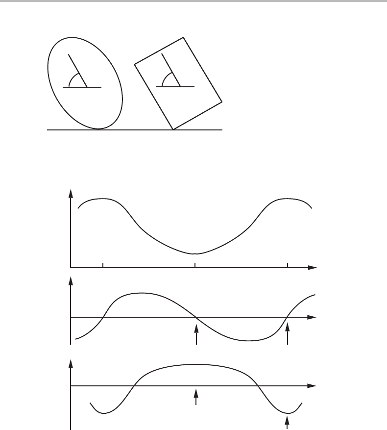
As an introduction to a more detailed discussion of stability it may be instructive to

compare with the mechanical analogues in Fig. 6.1.Itshows two bodies with different

cross-sections and in contact with a ﬂat ﬂoor. Their potential energy varies with the

angle θ.

Only very slow changes will be considered, and it will be assumed that any release of

potential energy goes into frictional losses. Kinetic energy will thus be neglected. The

extent of the process, ξ, will be expressed by the angle θ and the potential energy will

be denoted by E.

The variation of E, D and B with θ is illustrated in Fig. 6.2 for the body with an elliptical

proﬁle. It has an energy minimum at θ = 0 and a maximum at θ = π/2. In both these

positions the driving force for a further rotation is zero, D =−dE/dθ = 0, and they

both represent equilibria. The quantity d

E/dθ

=−dD/dθ may there be regarded as

the stability and the lower part of the diagram shows that for θ = 0itispositive and

the equilibrium is thus a stable one. For θ = π/2itisnegative and the equilibrium is

unstable. A small ﬂuctuation of θ away from π /2 in any direction will here give a force

for a further growth of the ﬂuctuation.

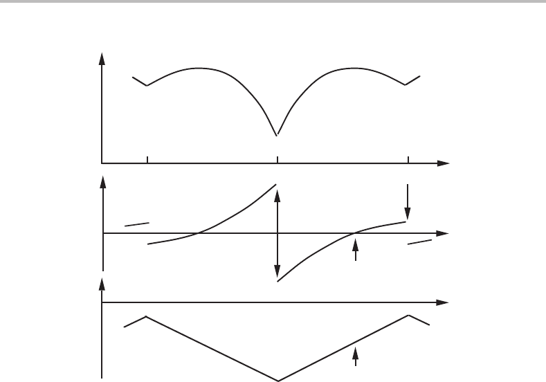
Figure 6.3 is for the body with a rectangular cross-section. It also has two equilibria,

at θ = 0 and π/2, which are both stable because a small ﬂuctuation of θ will give a force

for rotation back to the initial position. This case corresponds to Fig. 1.6 where 

S has

6.1 Introduction 109

Figure 6.1 Mechanical analogues of two cases of thermodynamic systems.

equilibrium equilibrium

π/2

−π/2 0

Potential

energy E

Driving force

D =−dE /dθ

Stability

B = 2d

E/dθ

This equilibrium

is stable

This equilibrium

is unstable

Figure 6.2 The energy, driving force and stability for the elliptical body in Fig. 6.1 as function of

the angle of rotation.

a sharp maximum. In order to decide whether such an equilibrium is stable it is not only

unnecessary but even incorrect to look at the value of d

E/dθ

because it represents

the stability only when the driving force is zero, D =−dE/dθ = 0, which is not the

case for θ = 0orπ/2. Figure 6.3 demonstrates that d

E/dθ

would give an incorrect

prediction for these two equilibria. On the other hand, there is a third equilibrium which

has D =−dE/dθ = 0atsome angle between 0 and π /2 and there d

E/dθ

< 0 and

will correctly predict that the equilibrium is unstable.

110 Stability

equilibrium

π/2

−π/2 0

stable

equilibrium

metastable

equilibrium

This equilibrium

is unstable

Potential

energy E

Driving force

D =−dE/dθ

Stability

B = 2d

E/dθ

Figure 6.3 The energy, driving force and stability for the rectangular body in Fig. 6.1 as function

of the angle of rotation.

Of the two stable equilibria, one (θ = π/2) has a higher energy than the other (θ = 0).

For thermodynamic systems such a state is called metastable.

6.2 Some necessary conditions of stability

In the discussion of general conditions of equilibrium in Section 1.10 we saw that a

system is in a state of internal equilibrium with respect to the extensive variables if

each one of the potentials has the same value in the whole system. It remains to be

tested if it is a stable or unstable equilibrium. We thus return to the combined law

according to the energy scheme and apply dU to the whole system, but we replace Ddξ

in Eq. (1.54)by−

B(dξ)

because we shall only consider a state of equilibrium where

D = 0.

dU = Y

B(dξ)

. (6.2)

First we shall consider only one internal process at a time, the transfer of dX

from

one half of the system, denoted by



,tothe other, denoted by



,dξ = dX



=−dX



On the other hand, we shall limit the discussion to systems with no exchanges with the

6.2 Some necessary conditions of stability 111

surroundings. All the dX

of the total system are zero and Eq. (6.2) simpliﬁes to

dU =

B(dξ)

(6.3)

B =

∂

∂ξ



∂

(∂ X

)







∂

(∂ X

)





. (6.4)

Here we have used the fact that the change of U in the total system must be equal to the sum

of the changes in the two subsystems. The two terms are equal if the system consists of a

homogeneous substance at equilibrium. By introducing the potential Y

= (∂U/∂ X

)

we then obtain

B =

∂

∂ξ

= 2



∂

(∂ X

)





= 2



∂Y

∂ X





. (6.5)

The value of this derivative depends upon the size of the system. It should be evaluated

for half of the system but the stability condition, B > 0, is not affected by the size. The

derivative may thus be evaluated for a system of any given size in the formulation of the

stability condition. It can be written as



∂

(∂ X

)



> 0or



∂Y

∂ X



> 0orU

> 0. (6.6)

The last form uses the shorthand notation for derivatives of characteristic state functions,

introduced in Section 2.5.

From Eq. (6.6)wemay conclude that in order for a substance to be stable it is necessary

that it has such properties that any pair of conjugate variables must change in the same

direction if all the other extensive variables are kept constant. Actually, so far we have

proved this only for conjugate pairs appearing on the energy scheme, i.e., (T, S), (−P, V )

and (µ

, N

). For them the stability conditions could be written as

> 0; U

> 0. (6.7)

As an example, in a stable system the chemical potential of a component, µ

, cannot

decrease when the content of the same component, N

, increases under constant S and

V.Asanother example, when the temperature of a substance is increased at a constant

volume, the entropy must also increase in order for the system to be stable.

≡



∂T

∂ S



V,N

> 0. (6.8)

Using Eq. (2.27)wecan write this stability condition as

T/C

> 0. (6.9)

In combination with the fact that the absolute temperature T is always positive, this

implies that the heat capacity under constant volume, C

, must be positive

= T (∂ S/∂T )

V,N

= T /(∂ T/∂ S)

V,N

> 0. (6.10)

112 Stability

However, in order to indicate where the limit of stability is, one should stick to the

condition as obtained directly from Eq. (6.8), i.e Eq. (6.9), or since T is positive,

1/C

> 0. (6.11)

The limit of stability occurs as 1/C

goes to zero, i.e., as C

goes to inﬁnity. Similar

considerations can be based upon the entropy scheme, where we have

− dS = (−1/ T )dU + (−P/T )dV + (µ

/T )dN

− (D/T )dξ. (6.12)

By again replacing Ddξ at equilibrium by −

B(dξ)

we obtain under constant U, V

and N

−dS =

(dξ)

(6.13)



∂

(−S)

∂ξ





∂

(−S)

∂(X

)







∂

(−S)

∂(X

)





= 2



∂Y

∂ X





. (6.14)

Since T is never negative, we ﬁnd



∂Y

∂ X



> 0, (6.15)

where X

, Y

is any pair of conjugate variables appearing in the entropy scheme, i.e.

(−1/T, U ), (−P/T, V ) and (µ

/T, N

). As an alternative we could have deﬁned the

stability by replacing (D/ T )dξ with −

B(dξ)

. Then T would not have appeared in

Eqs (6.9) and (6.10). Similar considerations can also be based on the volume scheme

introduced in Section 3.5,

dV = (T /P)dS − (1/P)dU + (µ

/P)dN

− (D/P)dξ. (6.16)

At equilibrium under constant S, U and N

it yields

= 2



∂Y

∂ X





. (6.17)

The conjugate pairs of variables are here (T /P, S), (−1/P, U ) and (µ

/P, N

Exercise 6.1

In Section 2.7 we saw that Gr¨uneisen’s constant can be evaluated from γ = V (∂ P/∂U)υ

and it often has a value of about 2. Is this a quantity that is always positive for a stable

system?

Solution

γ concerns the variation of P with U but they are not conjugate variables in any of the

schemes presented in Table 3.1. Thus, we cannot prove that γ is always positive. On the

contrary, it may be negative because α may be negative in rare cases and γ = V α/κ

6.3 Sufﬁcient conditions of stability 113

6.3 Sufﬁcient conditions of stability

So far we have discussed stability with respect to one internal process at a time. In

Chapter 5 we considered more than one simultaneous process, expressing d

S as  X

dξ

or T d

S as  D

dξ

.Atequilibrium the forces are zero and we need the next higher-order

terms. Instead of Eq. (6.1)weshould write

T d

S =



dξ

−



dξ

=−



dξ

. (6.18)

We should thus generalize Eq. (6.2) and by arranging the Y

terms in a special order

we write the combined law as

dU = T dS − PdV +µ

+···+µ

+ µ



dξ

(6.19)

We shall again keep all the extensive variables for the whole system constant and consider

the transfer of some amounts of the extensive quantities, here S, V , N

, N

,...,N

, N

between the two subsystems. In order for the system to be in a stable equilibrium all

the stability conditions given in Eq. (6.7) must be satisﬁed. However, in Chapter 5 we

found that cross terms could be very important for the kinetics and it is also true here.

It is an interesting question if it is then necessary to stipulate that all the B

stabilities

are positive in order to ensure that the system will be stable. In fact, it will now be

shown that it is sufﬁcient to ensure that a smaller set of conditions are satisﬁed if the

members of that set are chosen in a particular way. For the present set we have the

deﬁnition

∂

∂ξ

dξ

∂

∂ X



∂Y

∂ X



(6.20)

According to Section 2.5, B

could be denoted U

because the set of extensive

variables are the natural variables of the U.

By ﬁrst considering the transfer of only some amount of one of the extensive variables,

there will be no cross effects and taking the ﬁrst extensive variable we write

≡



∂T

∂ S



V,N

,...,N

> 0, (6.21)

as a condition of stability. Next, consider the transfer of dV but also of some S.However,

it is possible to eliminate the cross effect between them by the use of the combined law

after subtracting d(TS),

dF = d(U − TS) =−SdT − PdV + µ

+···+µ

+µ



dξ

. (6.22)

Instead of prescribing the amount dS to be transferred we shall consider the amount

that keeps T constant. The value of T, being a potential, must be uniform in the system

114 Stability

at equilibrium and there can be no cross terms between a potential and an extensive

quantity. The new stability condition will simply be



∂(−P)

∂V



T,N

,...,N

> 0. (6.23)

Next we shall add d(PV) obtaining dG and when considering the transfer of dN

the

next stability condition in the set will be



∂µ

∂ N



T,P,N

,...,N

> 0. (6.24)

Then we subtract d(µ

) obtaining a characteristic state function applied in Eq. (3.44),

d(G − µ

) =−SdT + V dP − N

dµ

+ µ

+···

+µ

+ µ



dξ

. (6.25)

When considering the transfer of dN

we obtain the stability condition

(G − µ

)



∂µ

∂ N



T,P,µ

,...,N

> 0. (6.26)

By proceeding in the same way we obtain conditions involving all the components from

2toc and each time with one more potential among the variables that are kept constant.

Finally we obtain



∂µ

∂ N



T,P,µ

,...,µ

c−1

> 0. (6.27)

It would seem that there is one more derivative in this series, (∂µ

/∂ N

)

T,P,µ

,...,µ

where all the variables to be kept constant are potentials. However, that derivative is

always equal to zero in view of the Gibbs–Duhem relation between the potentials. It says

that µ

cannot vary if all the other potentials are constant. The ﬁnal derivative thus yields

a trivial condition, which will not be included in the set of stability conditions.

We have thus been able to derive a set of c + 1 stability conditions without involving

any cross terms. As explained in more detail in Chapter 8,atequilibrium there are

c + 1degrees of freedom in a one-phase system with c components. The set of c + 1

stability conditions can thus ensure that the system with its c + 1degrees of freedom is

stable against all possible ﬂuctuations that can utilize the c + 1degrees of freedom. We

have thus obtained a sufﬁcient set of stability conditions. Naturally, one could form a

number of such sets by rearranging the extensive variables in a different order. It should

be emphasized that if all the conditions in a sufﬁcient set are satisﬁed, then all other

stability conditions are automatically satisﬁed. It may be mentioned that the variable, put

last among all the extensive variables, was thus chosen to express the size of the system.

For that purpose Gibbs used the volume V.Ofcourse, any extensive variable could be

used.

Finally, it should be emphasized that a set of stability conditions can only be sufﬁcient

with respect to the particular kinds of freedom that are considered. In addition to those

considered so far, there could be degrees of freedom concerning the homogeneous state