Heard D.E. (editor) Analytical Techniques for Atmospheric Measurement

Подождите немного. Документ загружается.

232 Analytical Techniques for Atmospheric Measurement

such as organic chemistry and physics. The first commercially available mass spectrometer

with magnetic sector mass filter was delivered in 1942 for the purpose of analysing

synthetically prepared organic compounds. Further developments quickly followed,

particularly in mass filters and detectors. The time of flight mass spectrometer (see

Section 5.3.2.2), quadrupole analyzer (Section 5.3.2.1) and the ion trap (Section 5.3.2.4)

were developed in the 1950s, and with the advent of the first computers systems became

more automated. The successful coupling of gas chromatography and mass spectrometry

improved the detection limits considerably, and as more commercial systems became

available in the 1960s, the technique proliferated throughout the field of science.

Mass spectrometers were first applied to atmospheric research in the 1960s. This work

was stimulated by the discovery that radio waves are reflected in the ionosphere and

a desire to understand the atmospheric distribution of ions. We now know that ions

are produced naturally in the atmosphere and their concentration controls the electrical

properties of the atmosphere as well as influencing important processes such as aerosol

production. Cosmic rays comprising extraterrestrial protons and alpha particles impinging

on the earth have sufficiently high energy to ionise N

(15.58 eV) and O

(12.07 eV).

Being charged, the resulting ions are affected by the earth’s magnetic field, analogously to

those in the mass spectrometer described above. The radiative emission of these particles

is the source of the Aurora seen at high latitudes. Over the first 100 km of the atmosphere

the ionisation density is relatively constant, around 10

ions cm

−3

. Since the neutral gas

density varies by a factor of 4×10

in this range, the mixing ratio of ions to neutrals

decreases substantially from high altitude to low altitude. At the surface there is only

one ion for circa 10

neutral molecules and the only significant source is from radon

(Viggiano & Arnold, 1995). Interestingly, for the reasons given above, the use of mass

spectrometry in the atmosphere began not at the ground but at high altitude (Narcisi &

Bailey, 1965). This was partly due to the interest in the ionosphere but mostly because

the high ion-to-neutrals ratio made it technically easier to make these measurements in

this region despite the inherent difficulty in getting the instruments to 60–100 km above

the Earth (see Section 5.2.1). Indeed it was only much later that the first measurements

of atmospheric ions were made from aircraft in the troposphere (Heitmann & Arnold,

1983), and then at ground level (Perkins & Eisele, 1984). Only positive atmospheric

ions were measured until 1971. In 1971, negative atmospheric ions were first measured

using rocket and balloon borne instruments (Arnold et al., 1971). This group discovered

that mass spectrometric measurements of naturally occurring ions in the middle to

lower atmosphere also provided information on the neutral trace gas composition (e.g.

acetone). It was a natural step to extend the measurement apparatus to include an

internal ion source, leading to the development of the atmospheric pressure ionisation

chemical ionisation mass spectrometer (API-CIMS) technique (see Section 5.4.1), based

on the principle of chemical ionisation first demonstrated by Munson and Field in 1966.

Through the 1980s these techniques permitted the measurement of important trace gases

in the upper troposphere and stratosphere. Airborne nitric acid measurements over the

Antarctic significantly contributed to the understanding of ozone hole chemistry. In the

laboratory, the improved sensitivity of continuous flow GC-MS allowed isotope ratios

of many important species to be determined (Barrie et al., 1984). In the 1990s chemical

ionisation mass spectrometry was developed for the measurement of important radical

species such as OH in the lower atmosphere. Despite its low concentrations and reactivity,

Mass Spectrometric Methods for Atmospheric Trace Gases 233

this species is now routinely measured at Hohenpeissenberg, Germany (see Figure 5.2).

The capillary GC-MS has become the most widespread MS technique in atmospheric

research, being particularly suited for measurement of organohalogens, CFCs, HCFCs

and alkanes. In 2000, the proton transfer reaction mass spectrometry technique became

commercially available and has proved popular for measurements of selected oxygenates

on short time scales (e.g. methanol). The number of atmospheric species measured by

mass spectrometry continues to increase, while detection limits, sampling time, size and

weight of instrumentation decreases. Within a century, mass spectrometry has developed

from a single laboratory experiment to become the most powerful and prolific technique

in atmospheric trace gas research at the time of writing, being applied from the tropics

to the poles and from the ground to the top of the atmosphere. Several examples of the

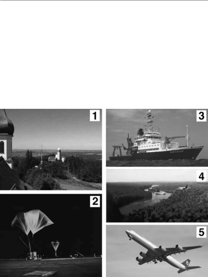
application of mass spectrometry in atmospheric field studies are given in Figure 5.2.

Figure 5.2 Examples of where trace gas mass spectrometry is used in atmospheric science.

(1) Ground-based APICIMS at Hohenpeissenberg for the routine measurement of OH. http://www.dwd.

de/en/FundE/Observator/MOHP/MOHP.html.

(2) Balloon launch of mass spectrometer to stratosphere from Kiruna, Sweden (Arnold & Henschen, 1978).

(3) The German research ship Meteor carrying PTR-MS and GC-MS measurements (Williams et al., 2004).

(4) Aircraft flying PTR-MS over the Amazonian rainforest (Crutzen et al., 2000).

(5) Commercial passenger aircraft carrying mass spectrometers and taking air samples on a regular basis for

long-term monitoring of the atmosphere (http://www.caribic-atmospheric.com/).

234 Analytical Techniques for Atmospheric Measurement

5.2 Fundamentals

5.2.1 The importance of vacuum

In Section 5.1 we have described mass spectrometry as involving the selective manip-

ulation of ions to a detector by electric and magnetic fields. Accurate deflection of

ions can only be achieved at low pressures as otherwise frequent collisions with neutral

molecules would destroy the order in the trajectories and possibly produce unwanted

ion–molecule reactions. Thus vacuum is essential for mass spectrometric analysis. From

kinetic theory the mean free path (L in m) of an ion at room temperature and pressure

can be calculated by:

L =

√

2 ×p ×

(5.1)

Where k is the Boltzman constant 1381×10

−23

−1

, T is the temperature (in K), p is

the pressure (in Pa) and  is the collision cross section (typically 50×10

−20

). For mass

spectrometry a mean free path of circa 1 m is required, generally somewhat longer than

the mass filter. It follows that the maximum pressure should be 66 ×10

−3

Pa (66 nbar).

Furthermore, where high voltages are used in ion sources or mass filters, the pressure

must be further reduced to prevent arcing.

For the reasons given above, the invention of reliable and effective pumping methods

was key to the development of mass spectrometry, see Table 5.1. This is normally done

in two steps. First, a mechanical pump is used to reduce the pressure from ambient

pressure 1 bar 10

Pa to around a millibar 10

Pa. Nowadays clean diaphragm pumps

are preferred in place of the older rotary oil sealed pumps. To achieve high vacuum

(better than a millibar) an alternative pumping principle to that of compression must be

used. For this a diffusion pump is the simplest form; however, in modern instruments

these are being superseded by turbo molecular pumps. The later consist of several stages

of fast rotating blades (typically 60 000 rpm) that drive molecules to a mechanical pump.

Since the molecular pumps cannot operate at near ambient pressure they must be used in

combination with a mechanical pre-pump. When used to analyse ambient air in the field,

care must be taken to ensure that pumps are not shaken or vibrated excessively. This is

particularly true for the fast-rotating turbo pumps. When operated on aircraft or ships,

pumps are often mounted on shock-absorbing mounts or the entire mass spectrometer

is switched off before landing to prevent damage.

5.2.2 The atomic mass scale

Atomic and molecular weights used in mass spectrometry are generally expressed in terms

of atomic mass units (amu) or daltons. This unit is based on a relative scale in which the

reference is the carbon isotope

C, which has been assigned the mass of exactly 12 amu.

Therefore, by definition, 1 amu is 1/12 of the mass of one neutral

C atom.

1 amu =1 dalton = 1/1212 g

C/mol

C/60221 ×10

atoms

C/mol

C

= 166054 ×10

−24

g/atom

C =166054 ×10

−27

kg/atom

Mass Spectrometric Methods for Atmospheric Trace Gases 235

The atomic weight of an isotope such as

Cl is related to the reference

C by comparing

the two masses. Since the chlorine isotope is 2.914707 times heavier than that of the

carbon isotope the mass of the chlorine isotope is:

Cl =120000 dalton ×219407 =349688 dalton

As 1 mol of

C weighs 12.0000 g, the atomic weight of

Cl is 34.9688 g/mol.

One result of this relative scale is that the masses of most ions in a mass spectrum fall

near but not at integer values. Acetone (propanone), for example, has an exact mass of

58.0418.

3 ×120000 +6 ×100783 +1 ×1599491

CHO

Table 5.2 gives the exact masses of a selection of isotopes of common elements and

selected atmospheric trace gas species.

Note that for stoichiometric calculations, chemists use the average mass calculated using

the atomic weight, which is an average of the isotopes of each element of the molecule. The

average mass of methane would therefore be 1201115 +4 ×100797=160434 daltons

(see Table 5.2). However, in mass spectrometry, the monoisotopic mass generally is

used. This mass is calculated by using the mass of the most abundant isotope for each

constituent element. Methane is therefore 120000 +4 ×100783 = 1603132 daltons. In

mass spectrometry we may need to distinguish between ions with almost identical masses.

The extent to which they can be differentiated depends on the resolution of the mass

Table 5.2 Exact masses of selected elements and molecules

Element Atomic mass/daltons

H 1.00783

H 2.01410

C 12.00000

C 13.00335

N 14.00307

N 15.00011

O 15.99491

O 17.99916

Cl 34.96590

Cl 36.96590

68.06264

N 67.04222 (Low resolution needed)

COCH

58.0418

HC(O)CH(O) 58.00548 (Medium resolution needed)

D 17.03758

17.03466 (High resolution needed)

236 Analytical Techniques for Atmospheric Measurement

spectrometer. In Table 5.2 the masses are given with four or five figures to the right of

the decimal point. High resolution mass spectrometers have this precision.

As has been noted above, ions are required to perform mass spectrometry. How these

ions interact with applied electric and magnetic fields depends on the mass and the

charge of the ions. It is important to note that a mass spectrometer determines the

mass-to-charge ratio m/z of these ions, see Figure 5.1. For example, singly charged

methane

, has m/z = 1603132 whereas

has m/z =8518. Where z is the

total charge of the ion Q divided by the charge of one electron e:

z = Q/e e =16 ×10

−19

Coulomb (5.2)

If mass is given in daltons and charge is given in electron charges, m/z is given in

thomson (Th). In some cases the unitless terms mass number and charge number are

given, in which case m/z is also unitless. Most ions encountered in mass spectrometry

have a charge corresponding to the loss of one electron. For this reason the term ‘mass-

to-charge ratio’ is often shortened to mass.

5.2.3 Resolving power and resolution

The resolving power of a mass spectrometer is a measure of its ability to separate two

ions of any defined mass difference. The theoretical resolving power necessary to separate

two ions differing in their m/z is defined as M/M, where M is the mean of the two

masses and M is the difference between the two masses. In order to separate an ion

of the major biogenic emission product isoprene m/z 68 from an ion of the biomass

burning product pyrrole m/z 67 a theoretical resolution of about 68 is required. This

is considered to be low resolving power. A medium resolving power of circa 1600 is

required to resolve the atmospherically important molecule acetone m/z 5804186 from

the shorter-lived whole mass isomer glyoxal m/z 5800547 (see Table 5.2). Note that

the isomers acetone and propanal have exactly the same mass and therefore cannot be

resolved. Methane is an important trace gas in the atmosphere and valuable information

about its sources and sinks can be obtained by measuring its isotopes. This is complicated

as the methane isotopes

and

D require a mass spectrometer with higher

resolving power, in this case ca. 5800. The original mass spectrometer built by Thomson

had a resolving power of about 13 which was improved tenfold by his student Aston in

1933, see Table 5.1. Commercial mass spectrometers are available with resolving powers

from a few hundred to 500 000.

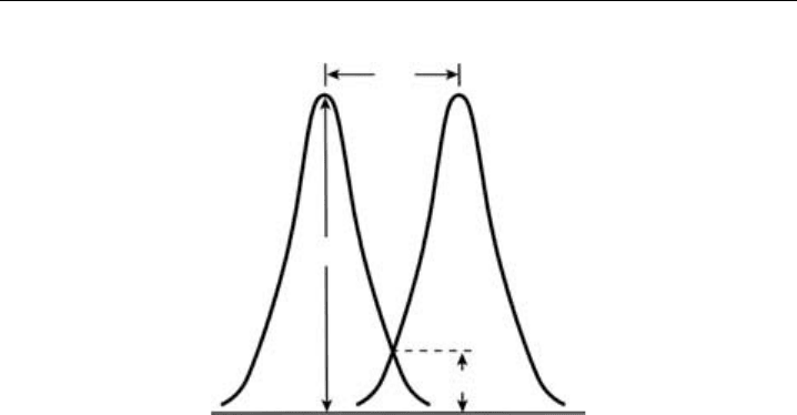
In Figure 5.3, two overlapping mass peaks M

and M

in a mass spectrum are depicted.

The resolving powers calculated above do not specify the acceptable degree of separation

between the ions with slightly different masses. This is given by the resolution R, which is

defined as the smallest mass difference for which two masses (M

and M

) are resolved. By

general agreement the peaks M

and M

are said to be resolved if the height of the valley

between the peaks h is equal or less than 10% of the peak height H. The resolution R

therefore defines the smallest mass difference M of peak width for which the two peaks

and M

are resolved to this extent. Many quadrupole instruments operate at constant

Mass Spectrometric Methods for Atmospheric Trace Gases 237

ΔM

Figure 5.3 Parameters deﬁning peak resolution.

resolution. This means that the ability to separate mass 100 and mass 1000 is the same.

Note that if the resolution M is 1 amu at m/z =100, then the resolving power is 100.

However if M is 1 amu at m/z = 1000, then the resolution is still one but the resolving

power is 1000. In practice, the resolution may be set by introducing compounds at a

suitable mixture into the mass spectrometer to generate peaks M

and M

. Adjustment of

the various operating parameters of the mass spectrometer is performed until the peaks

have the desired resolution, i.e., 10% valley. Since sometimes it is difficult to get two

mass spectral peaks of equal height adjacent to one another, an alternative method of

calculating M is to use the full width at half maximum (FWHM) of a single m/z value

peak. Resolving power calculated using the FWHM method gives values for R that are

about twice that determined by the 10% valley method. By determining the resolving

power by using the full width at 5% full maximum, an R value close to the 10% valley

method can be derived. However, this is very difficult in practice because of background

signals.

5.3 Key elements of a mass spectrometer

5.3.1 Ionisation

The first step in the mass spectrometric analysis of an air sample is the ionisation of the

sample. The method used to ionise a substance profoundly influences the appearance of

its mass spectrum. For trace gas species in ambient air, two methods of ionisation are

currently prevalent. These are termed ‘electron ionisation’ and ‘chemical ionisation’ and

discussed in Sections 5.3.1.1 and 5.3.1.2 respectively.

238 Analytical Techniques for Atmospheric Measurement

5.3.1.1 Electron ionisation

Electrons produced from a heated filament in an evacuated chamber can be accelerated

towards an anode by applying a voltage (V). The energy of these electrons will be eV,

where e is the charge of the electron. Each electron is associated with a wave whose

wavelength ,

 =

(5.3)

where m is its mass, v is its velocity and h is Planck’s constant. For kinetic energies of

70 eV the wavelength is 14 ×10

−10

m. When this wavelength is close to the bond lengths,

the electron waves and the electric field of the molecule mutually distort one another. The

distorted electron wave can be considered to be many waves with different frequencies

and if one of the waves has the correct frequency (or energy) to interact with molecular

electrons (i.e. the energy corresponding to a transition), an energy transfer can occur. The

interaction of an electron with a molecule is rather non-specific. One possibility is that

the molecule may be electronically excited, in similar fashion to ultraviolet spectroscopy

(see Chapter 3). This can be represented by

M +e →M

∗

−

(5.4)

Alternatively a molecular electron may be ejected from the molecule to leave a radical

cation. This is the best outcome for subsequent mass spectrometry since it produces an

ion that can be manipulated in electric and magnetic fields.

M +e

−

→ M

·+2e

−

(5.5)

A further possibility is direct capture of the electron by the molecule to give a stable

radical anion. However, the probability of this is low. Although less than one per cent

of the sample molecules are converted to positive ions, electron capture as depicted in

Equation (5.6) is probably one hundred times less probable.

M +e

−

→ M

−

· (5.6)

The energy of the ionising electrons may be varied by varying the applied voltage.

By convention, standard mass spectra are obtained at 70 eV since the maximum ion

yield is obtained near this energy. Furthermore, at this level small changes in energy

do not greatly affect the mass spectrum, helping the reproducibility of the analysis.

Mass spectra can be obtained at any electron energy above the ionisation energy of the

molecule (typically between 6 and 12 eV). Indeed it is often desirable to measure the

mass spectrum at energy levels less than 70 eV, despite the reduction in ion abundance,

since the amount of molecular fragmentation following ionisation can be reduced and

therefore identification facilitated. At higher potentials the electron wavelengths become

too small and molecules become effectively transparent. Extensive mass spectral libraries

Mass Spectrometric Methods for Atmospheric Trace Gases 239

have been compiled for substances ionised by electron ionisation at 70 eV. These can be

matched against unknown spectra from a sample to identify components.

5.3.1.2 Chemical ionisation

In chemical ionisation, ions are produced through the collision of the molecule to be

analysed with primary ions present in the source. The indirect method of chemical

ionisation (CI) is a complementary technique to the direct method of electron ionisation

(EI). While the high energies involved in EI commonly lead to fragmentation of the

molecular ion, chemical ionisation produces ions with little excess energy. Less fragmen-

tation facilitates identification of molecular species. Ion sources for chemical ionisation

are very similar to those for EI but they typically operate at high pressures (e.g. 0.1 mbar

compared to 10

−6

mbar for EI). In other words, in EI the gas sample is reduced in

pressure before the ionisation directly before the mass filter, while in CI the ionisation

generally occurs at higher pressure but the resulting ions must be directed via ion lenses

to the low pressure region containing the mass filter. In CI, both positive ions (e.g.

ions) and negative (e.g. SF

−

ions) can be used. Reactant gas ions are created by

leaking a reactant gas into an ion source where they interact with an electron beam or

high energy particles (e.g. emitted by radioactive sources) to produce primary ions. The

pressure in the ionisation region is adjusted so that the concentration ratio of reagent

to sample is 10

–10

. Because of this large concentration difference the electron interacts

predominantly with the reagent. The reagent ions then react with the sample molecules

of interest to produce ions. This form of chemical ionisation has two advantages over

electron ionisation described in Section 5.3.1.1. First, electron ionisation of a molecule

can give rise to a multitude of fragments, and for a complex mixture like ambient

air, the resulting mass spectrum can be indecipherable. Secondly by judiciously choosing

the reagent ion the trace gases of interest in the air can be detected preferentially over

the hugely more abundant species such as nitrogen and oxygen. Typical reagents are

methane, water and ammonia. Water is used for measurement of species such as acetone

by API-CIMS and PTR-MS (Sections 5.4.1 and 5.4.2). Methane has been used in negative

ion chemical ionisation in combination with gas chromatography, for the analysis of alkyl

nitrates and organohalogens in air (Section 5.4.4).

5.3.2 Mass ﬁlters

The mass filter is the heart of the mass spectrometer. It is here that the ions that have

been produced in the ion source are separated according to their m/z. The ability to

separate ions is characterised by the resolution (see Section 5.2.3). From the geometrical

configuration of the mass filters described below a theoretical resolution can be calculated.

However, in all cases the actual resolution is dependent on many other factors specific to

the device in question (e.g. constancy of the electric fields etc.) and should be empirically

assessed. The mass filters described below are all used in atmospheric research. In this

section the principle of each is described and in Sections 5.4 and 5.5 various applications

of these filters are described.

240 Analytical Techniques for Atmospheric Measurement

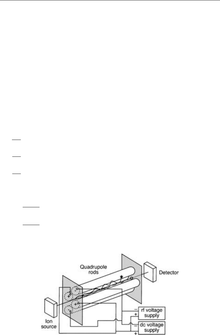
5.3.2.1 Quadrupole

The quadrupole mass filter is a device that uses the stability of the trajectories in oscillating

electric fields to separate ions according to their m/z, see Figure 5.4. An ideal quadrupole

consists of four symmetrically arranged hyperbolic shaped surfaces of infinite length. In

reality, quadrupole mass filters consist of four parallel cylindrical rods. Typically these

are 10–20 mm in radius and 20 cm long. Opposing rods are electrically connected and a

potential comprising a DC voltage U  and an RF component V ·cos t is applied. For

example when a positive ion enters the space between the rods, the electric field will act

to draw it to a negative rod. If the rod potential changes sign before the ion discharges

on the rod, the ion will change direction. Since there is no field applied in the z axis the

ions continue with the same speed as they enter the quadrupole. The DC and RF fields

can be varied so that an ion of a specific m/z can pass through the rods while others

do not.

The equations of motion of an ion in a quadrupole can be represented by the Mathieu

differential equations:

+ a +2q cos t =0 (5.7)

− a +2q cos ty = 0 (5.8)

= 0 (5.9)

where,

a =

8eU



(5.10)

q =

4eV



(5.11)

t = 2 (5.12)

Figure 5.4 A schematic diagram of a quadrupole mass ﬁlter.

Mass Spectrometric Methods for Atmospheric Trace Gases 241

The solutions to these differential equations lie in two classes, corresponding to either

‘stable’ or ‘unstable’ trajectories. When the rod potentials (U, V and/or ) are varied in

a suitable manner then an ion of selected m/z (and only this ratio) may pass through the

quadrupole to the detector. By adjusting these potentials with time to satisfy a small mass

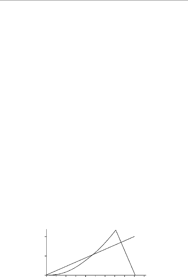
and then sequentially the larger masses, a mass spectrum can be generated. Figure 5.5

shows a so-called stability diagram for a quadrupole. Within the area defined by the

shark’s fin triangle are values of a and q generating stable solutions. The operating line

of the quadrupole is defined by the ratio a/q = 2U/V . By increasing this ratio, the

region of stable solutions can be so restricted that only ions of a specific mass pass

through. In this way the resolution of the mass filter can be varied, i.e. higher the ratio

the higher the resolution. However, when too high a ratio is chosen, the operating line is

no longer secant of the stable area and no ions will pass at all. For a real quadrupole, the

efficiency of transmission of ions depends on the exact locations and directions of the

ions when entering the rod system. Ions entering the rod system inclined to the z-axis

may possibly not pass the filter despite having the correct m/z. In fact the transmission

in the mass filter (number of ions entering/number of ions exiting) is approximately

inversely proportional to the resolution. Both transmission and resolution can influence

the accuracy and precision of a measurement and a compromise must be made between

the two for optimum performance.

Quadrupole mass filters are often operated at unit mass resolution (i.e. 1 amu, low

resolution), in contrast to the magnetic mass filters described in Section 5.3.2.3. However,

quadrupoles are relatively cheap and easy to operate. This is because the necessary

electronics (precise RF generators) have become standard technology instruments.

5.3.2.2 Time of ﬂight

When ions of different masses are produced at the same place with the same energy, and

then accelerated by a potential V over a distance d, they will arrive at different times. The

time of flight mass filter relies on an accurate measurement of these times to distinguish

ions of different masses. In reality, ions are usually continually produced but expelled

in bundles from an ion source by the transient application of a potential to the source

0.2

0.1

Stable region

Unstable

region

Unstable

region

a/q = 0.15

0.0

0.0 0.2 0.4

0.6 0.8 1.0

Figure 5.5 The stability diagram for a quadrupole.