Hatano Y., Katsumura Y., Mozumder A. (Eds.) Charged Particle and Photon Interactions with Matter - Recent Advances, Applications, and Interfaces

Подождите немного. Документ загружается.

70 Charged Particle and Photon Interactions with Matter

where the Kohn–Sham Hamiltonian h

[n(t)] is given by

h n t

V d

n t n t

xcKS ion

[ ( )] ( ) ( , ) [ ( , )].= − ∇ + +

′

−

′

∫

r r

r rµ (4.18)

The

time-dependent density is given by

n t t

( , ) ( , ) .r r=

∑

(4.19)

The exchange-correlation potential μ

[n(t)] is a key quantity in the TDDFT. It can be a nonlocal

function of the time-dependent density n(r,t) in both space and time. If an accurate exchange-

correlation potential is adopted, we expect that the time-dependent density n(r, t) calculated by the

TDKS equation coincides with that in the exact many-body quantum theory. In practice, however,

we can at most employ an approximate one. Indeed, in the calculations below, we will employ a

simple adiabatic approximation in which the exchange-correlation potential employed to describe

the ground state properties is employed for the time-dependent dynamics as well. We will later mention

the

spatial dependence of the exchange-correlation potential.

obtain an expression for the polarizability in the TDDFT, we apply a perturbation theory to

the TDKS equation, expanding the Kohn–Sham Hamiltonian up to a linear order in the density

change around the density in the ground state. In the adiabatic approximation, we have

h n t h n d

h n

n t

KS KS

[ ( , )] [ ( )]

[ ( )]

( )

( , ),r r r

r= +

′

∫

δ (4.20)

where the functional derivative of the Kohn–Sham Hamiltonian, δh

/δn has the following form in

the

local-density approximation (LDA),

δµ

h n

e n

ks XC

[ ( )]

( )

[ ( )]

( ).

r r r

r r

′

−

′

+ −

′

(4.21)

The potential, (δh

/δn)δn(t), includes effects caused by a change of the electron density and is

called the dynamical screening potential. If we regard a sum of the external potential and the

induced potential as a perturbation, one may describe the response of the system in terms of the

density–density response function without two-body interaction, which we call the independent-

particle response function and we denote it as χ

(r, r′, t − t′). The density change is expressed as

δ χ

n t dt d t t V t d

h n

( , ) ( , , ) ( , )

[ ( )]

(

r r r r r r

′ ′ ′

−

′ ′ ′

′′

′

0 ext

′′

′′ ′













∫∫∫

−∞

)

( , ) .δn t

(4.22)

For a perturbation with a xed frequency, ω, we can again separate the time variable. Expressing

δn(r,t)

as δn(r,

ω)e

−iωt

and V

ext

(r,t) as V

ext

(r,ω)e

−iωt

, we have

δ ω χ ω ωn d V( , ) ( , , ) ( , ),r r r r r=

′ ′ ′

∫

0 scf

(4.23)

Time-Dependent Density-Functional Theory for Oscillator Strength Distribution 71

V V d

h n

scf ext

( , ) ( , )

[ ( )]

( )

( , ).r r r

rω ω

δ ω= +

′

∫

(4.24)

This

equation should be solved for δn(r,

ω)

at each frequency, ω.

explicit form of the independent-particle response function is given by

χ ω

φ φ φ φ

ε ε ω δ

φ φ φ

( , , )

( ) ( ) ( ) ( ) ( ) ( ) (

r r

r r r r r r

′

′ ′

− − −

′

i m m i

i m

i m m

rr r) ( )

unocc.occ.

ε ε ω δ

i m

′

− + +













∈∈

∑∑

(4.25)

where ϕ

and ϕ

are occupied and unoccupied Kohn–Sham orbitals with eigenenergies ε

and ε

respectively.

They satisfy h

] ϕ

= ε

The dipole polarizability in the TDDFT may be dened in the same way as Equation 4.16. We

rst set the external potential as V

ext

(r,ω) = r

. Then δn(r, ω) is calculated by solving Equation 4.22

each frequency ω. We then obtain the polarizability by

α ω δ ω

µν µ

( ) ( , ).= −

∫

e d r n

r r

(4.26)

The oscillator strength function S(ω) can be dened in the same manner as Equation 4.9. We note

that the TRK sum rule is satised exactly in the TDDFT if one employs the adiabatic approxi-

mation for the exchange-correlation potential and if one solves the TDKS equation without any

approximation.

We can express the oscillator strength distribution as a sum of contributions of occupied orbitals

(Zangwill and Soven, 1980; Nakatsukasa and Yabana, 2001). We rst express the oscillator strength

distribution

as follows:

d V V

( )

( , ) ( , , ) ( , ).

ω χ ω ω

= −

′

∫

∑

2 1

r r r r r

scf scf

(4.27)

Then, noting that the independent-particle response function χ

(r, r′,ω) dened in Equation 4.25 is

written as a sum over occupied orbitals, one may decompose the oscillator distributions into orbitals.

4.2.4 exchange-correlation potential

In practical calculations, the choice of the exchange-correlation potential signicantly affects the

calculated oscillator strength distribution. In the TDDFT, we need to specify the frequency (time)

and the spatial dependence of the exchange-correlation potential. Regarding the frequency depen-

dence, we employ the adiabatic approximation, in which the exchange-correlation potential does not

depend on the frequency as mentioned above, because reliable frequency-dependent energy func-

tionals are not yet available. We employ the same exchange-correlation potential for both ground

state and response calculations. We also need to specify the spatial dependence of the exchange-

correlation potential. The simplest choice is the LDA, where it is assumed that the electrons at each

position behave as if they were in a uniform electron gas with the electron density at each point.

It has been known that even the LDA, the simplest functional, works reasonably for the oscillator

strength distribution. However, it is not accurate enough, especially around the ionization threshold.

It is well known that the spurious self interaction does not vanish in the LDA and, consequently, the

long-range −e

/r tail lacks in the LDA. Because of this failure, the magnitude of the orbital energy of

the highest occupied molecular orbital (HOMO) is much smaller than the ionization potential. Thus,

72 Charged Particle and Photon Interactions with Matter

the oscillator strength distribution around the ionization threshold cannot be described accurately in

the LDA. To remedy the failure of the LDA, a gradient corrected potential, the LB94, was proposed

(Van Leeuwen and Baerends, 1994). In the LB94, a term depending on the gradient of the density,

∇n(r), produces the potential that shows the correct asymptotic behavior. The ionization potentials

are also reproduced rather accurately. In our calculations presented below, we will employ the LB94

potential unless otherwise stated.

For an accurate description of low-lying excitations in molecules, assessment regarding the accuracy

of exchange-correlation potentials has been extensively achieved in quantum chemistry calcula-

tions. We quote a few references for such researches (Casida et al., 1998; Furche and Ahlrichs, 2002;

Dreuw

and Head-Gordon, 2005).

4.3 Computational details

The calculations of the oscillator strength distribution with the linear response TDDFT have

been rst achieved in the early 1980s for spherical systems, such as atoms and metallic clusters.

For spherical systems, χ

(r, r′,ω) dened by Equation 4.25 is a rotationally invariant kernel, and

Equations 4.23 and 4.24 for δn(r,ω) may be solved for each multipole component separately. The

equation for each multipole component is an integral equation of radial variable only, and can easily

be solved numerically. Also, the outgoing boundary condition for emitted electrons may easily be

incorporated

in the partial wave expansion for the wave functions.

For

systems without spherical symmetry, on the other hand, an explicit construction of the inde-

pendent-particle response function given by Equation 4.25 is numerically demanding, since it is a

function of two coordinate variables, r and r′. This is especially true in the Cartesian-coordinate

grid representation that we adopted here. For this reason, several efcient computational approaches

that avoid an explicit construction of the response function χ

have been developed. In this section,

outline briey the computational methods that we adopted in the calculations presented later.

4.3.1 real-Space grid repreSentation

To express orbital wave functions ψ

(r,t), we employ a three-dimensional Cartesian-coordinate grid rep-

resentation (Chelikowsky et al., 1994). We treat valence electrons explicitly, employing the so-called,

norm-conserving pseudopotential for electron–ion interaction (Troullier and Martins, 1991). We treat H

, N

, and O

as cores. The pseudopotential is further approximated to be a separable form, known

as the Kleinman–Bylander form (Kleinman and Bylander, 1982). This is a standard prescription in the

rst-principles DFT calculations with grid representation in either momentum or real-space grid repre-

sentation. We thus freeze the core electrons ignoring their polarization effects. The typical grid spacing

is 0.5 a.u.: this is ne enough to describe valence electron dynamics. We take grid points inside a cubic

box area. The typical size of the box is 60 a.u. in one side, which includes 120

grid points.

4.3.2 real-tiMe Method

The real-time method solving the TDKS equation in time domain is one of the straightforward ways

to calculate the polarizability of the whole spectral region (Yabana and Bertsch, 1996). As explained

in Equation 4.2, the dipole polarizability α

μν

(ω) is dened as a proportion coefcient between the

induced polarization, p

(t), and the applied external electric eld, E

(t), of a xed frequency, ω, applied

to ν-direction, E

(t) = E

−iωt

. Now let us consider an induced dipole moment p

(t) for an electric eld of

arbitrary time prole in ν-direction. In the linear response regime, each ω component of p

(t) and E

(t)

should be related by the dipole polarizability, α

μν

(ω), since there holds a principle of superposition,

dt e p t dt e E t

i t i tω

µ µν

α ω( ) ( ) ( ).=

∫ ∫

(4.28)

Time-Dependent Density-Functional Theory for Oscillator Strength Distribution 73

This relation tells us that for an applied electric eld of any time prole, we can calculate the dipole

polarizability

by taking the ratio of the Fourier transforms,

α ω

µν

( )

( ),=

∫



dt e p t

i t

(4.29)

where

(ω) is the Fourier transform of the applied electric eld,



E dt e E t

i t

ω( ) ( )=

∫

the practical calculation, we employ an impulsive dipole eld,

V t I t r

ext

( , ) ( ) ,r = δ

(4.30)

where I is the magnitude of the impulse. We assume that a molecule is in the ground state described

by the static solution of the DFT before applying the external potential at t = 0. The impulsive force

is then applied to all the electrons in the molecule at t = 0. In classical mechanics, each electron gets

an initial velocity ν = I/m by this impulse. In quantum mechanics, the same situation is described as

follows:

every orbital is multiplied by the plane wave with the momentum I.

ψ φ

iIr

t e( , ) ( ).

r r= =



(4.31)

We evolve the orbitals starting from this initial condition. During the time evolution, we do not

apply any external potential. The dipole moment is calculated by d t d r t

µ µ

ψ( ) ( , )=

∑

∫

r r

. The

Fourier

transform of the impulse eld is just the constant I. Then the polarizability is calculated by

α ω

µν

( ) ( ).=

∞

∫

dt e d t

i t

(4.32)

Since the impulsive eld includes the frequency components of the whole spectral region uniformly,

one may obtain the polarizability for the whole spectral region from a single time evolution calculation.

In the polarization function in time, p

(t), transitions to bound excited states appear as steady oscil-

lations that persist without any damping. However, the real-time evolution is achieved for a certain

nite period and, consequently, the Fourier spectrum of such oscillations shows wiggles around each

excitation energy because of the abrupt cut of the steady oscillations within a nite time period. The

wiggles may be diminished to some extent by introducing a damping function in the Fourier transfor-

mation of Equation 4.32. A simple choice for the damping function is the exponential function e

−γ t

Since this is equivalent to introducing a small imaginary part, iγ, in the frequency, this gives the bound

transitions a Lorentzian line shape if the time evolution is achieved for a sufciently long period.

Another choice is the damping function of a third order polynomial in time,

f t

( ) .= −

























1 3 2

2 3

(4.33)

Since

this function does not change the slope of p

(t) at t = 0, it does not change the TRK sum.

The typical time step is Δt = 0.027 a.u. We perform the time evolution for 5 × 10

time steps.

Thus, the total period of the time evolution is given by T = NΔt = 1350 a.u. The energy resolution

in the real-time calculation is determined by the inverse of the time period. In the present case, it

is ΔE = 2π/T = 0.13eV. We employ the width for smoothing, γ = 0.25 eV.

74 Charged Particle and Photon Interactions with Matter

4.3.3 treatMent of outgoing boundary condition for photoionization proceSS

To describe the photoionization process, we need to impose the scattering boundary condition for the

emitted electrons. For electrons emitted from a molecule, it is not at all obvious how to impose

the scattering boundary condition computationally. A lot of methods have been developed to treat the

problem. (See references in Cacelli et al., 1991; Nakatsukasa and Yabana, 2001.)

In the real-time calculation, the Kohn–Sham orbitals are distorted, by the impulsive external

potential. They include components corresponding to the unbound orbitals of the static Kohn–

Sham Hamiltonian. During the time evolution, electrons excited to the unbound orbitals are emitted

outside the molecule. Once the electrons are emitted outside the molecule, they never return to the

region around the molecule. They will not contribute to the transition density and to the polariz-

ability since the density change δn(r,t) only exists in the spatial region of the ground state density

distribution.

In the three-dimensional grid representation that we adopt in our calculation, we solve the TDKS

equation inside a certain box area. If we simply solve the equation, the electrons emitted outside

the molecule are reected at the box boundary and return to the region of the molecule. Then the

reected wave makes a standing wave in the region of the molecule and makes a spurious contribu-

tion to the polarizability. To describe the ionization process adequately, one must remove electrons

that

are emitted outside the molecule during the time evolution.

approximate removal of emitted electrons is feasible by placing a negative imaginary

potential outside the molecule. In the presence of the negative imaginary potential, the ux

is absorbed during the propagation. This is the so-called absorbing boundary condition. The

absorbing potential should be smooth enough so that the ux getting into the region of the

absorbing potential is not reected. On the other hand, the absorbing potential should be strong

enough so that all the ux is absorbed efciently. These two conditions may be satised if one

employs a sufciently long distance of absorbing potential. This, however, increases the num-

ber of grid points to be employed in the numerical calculation. We must nd a compromise of

these contrary conditions.

In the practical calculations presented below, we employ the absorbing potential with a linear coor-

dinate dependence. The potential is placed at a spatial region where the radial coordinate r is greater

than a certain radius R, beyond which the electron density in the ground state can be negligible.

Denoting the thickness of the absorbing region as ΔR, the absorbing potential is placed in the region

R < r < R + ΔR,

− =

< <

−

< < +











r R

R r R R

( )

0 0

∆

(4.34)

Here the height W

and the width ΔR must be carefully chosen. We adopt W

= 0.147 a.u. and ΔR =

18.9a.u. in the calculations presented below.

In the real-time method, the absorbing potential is simply added to the Kohn–Sham Hamiltonian

the time evolution,

t h n t iW V t t

i i

∂









− +

{ }

ψ ψ( , ) ( ) ( ) ( , ) ( , ).r r r r

ext

(4.35)

In the presence of the absorbing potential, the time evolution is no more unitary. However, since we

apply sufciently weak perturbation V

ext

(r,t), the loss of the ux by the absorbing potential is small.

We have found that the time evolution is stable for a sufciently long period to obtain the polarizability

with a desired accuracy.

Time-Dependent Density-Functional Theory for Oscillator Strength Distribution 75

4.4 osCillator strength distributions oF moleCules

We present the TDDFT calculations of the oscillator strength distributions for a variety of molecules.

We will show the calculations of small molecules, N

, O

, H

O, and CO

; several hydrocarbon mol-

ecules of small and medium size, acetylene, ethylene, benzene, and naphthalene; and a fullerene C

as an example of a large molecule. We will show that the TDDFT is capable of describing the overall

features of the oscillator strength distribution for all molecules studied. We will also show the decom-

positions of the oscillator strength distributions into occupied orbitals and clarify the character of the

discrete transitions. As the molecular size increases, the measured oscillator strength distributions

show fewer structures than those in the calculation. This should be due to the coupling of electrons

with molecular vibration that we ignored in the present calculation.

We make a comparison of our calculation with only a few measurements, usually the most

recently published values. We also quote only a few recently published calculations among many

others

in the past.

4.4.1 diatoMic and triatoMic MoleculeS

4.4.1.1 n

molecule

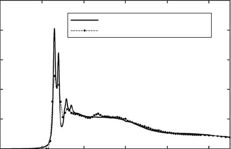
We show the TDDFT calculation for the oscillator strength distribution of N

molecule below 55eV

in Figure 4.1, in comparison with measurement (Chan et al., 1993a). The decomposition of the

strength into occupied orbitals is shown in Figure 4.2 for 10–20eV energy region. The calculated

energy of HOMO orbital is 15.63eV, which is in good agreement with the measured ionization

potential, 15.58eV. As seen from Figure 4.1, the overall features of the oscillator strength distri-

bution are nicely reproduced by the calculation. There are two transitions below the ionization

threshold. The transition at 13eV is composed of two transitions, from two orbitals, 3σ

and 2σ

The transition at 14eV originates mainly from the 1π

orbital. At around 16eV, there are two transi-

tions seen in the TDDFT calculation. Measurement shows a bump at around the energy. This mainly

comes from the 1π

orbital. At around 22 eV, the measurement shows a small bump. However, it is

not

visible in the TDDFT calculation.

similar TDDFT calculation has been presented by Stener and Decleva (2000), with a differ-

ent numerical method. The results presented here is consistent with those by Stener’s. Levine and

Soven (1984) also made a calculation of N

. Montuoro and Moccia (2003) made a calculation with the

K-matrix method.

0.8

0.6

0.4

Cal.

Exp. (Chem. Phys. 170 (1993) 81)

0.2

0 10 20 30

Energy (eV)

Oscillator strength distribution (eV

–1

)

40 50

Figure 4.1 Oscillator strength distribution of N

molecule. Solid line, TDDFT calculation; circles con-

nected

with dotted line, measurement. (Data from Chan, W.F. et al., Chem. Phys., 170, 81, 1993a.)

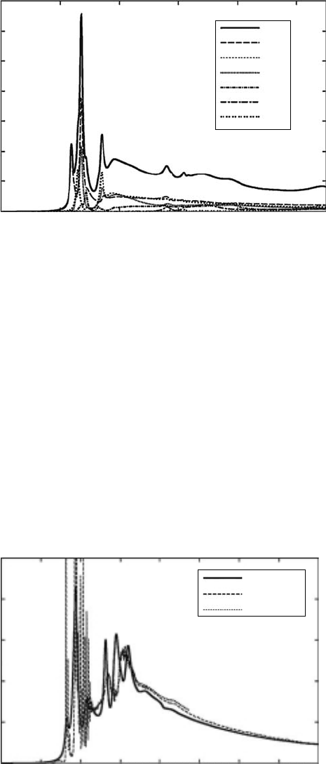
76 Charged Particle and Photon Interactions with Matter

4.4.1.2 o

molecule

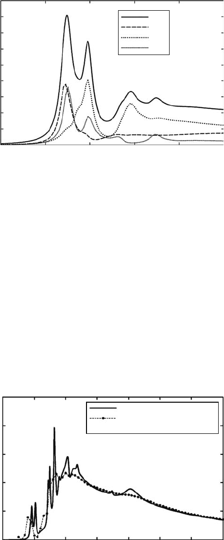
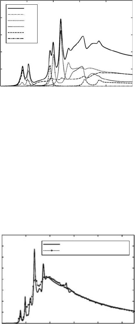
We show the TDDFT calculation for the oscillator strength distribution of O

molecule below 70eV in

Figure 4.3, in comparison with measurement (Brion et al., 1979). The decomposition of the strength

into occupied orbitals is shown in Figure 4.4 for 5–30eV energy region. The ground state of the O

molecule is spin triplet, the last two electrons occupy the two degenerate orbitals of 1π

aligning their

spin directions. However, in the present calculation, we ignore the spin structure, assuming that the

two degenerate 1π

orbitals of spin-up and spin-down are occupied equally by two electrons, 0.5 elec-

tron for each. We thus employ the energy functional with saturated spin structure. The energy eigen-

value of the HOMO is at 12.01eV, in good agreement with the measured ionization potential, 12.07eV.

Two transitions appear below the ionization threshold. They originate from the occupied orbitals of

1π

and 1π

. Above the threshold, three sharp structures appear at around 15eV in the calculation that is

mainly from 1σ

, 1π

, and 3σ

orbitals. However, in the measured spectrum, they are not well separated.

At around 35 and 40eV, the calculated oscillator strength shows a peak. In the same energy

region (40 eV), a slight bump is seen in the measured spectrum. In the calculation, these peaks come

0.9

0.8

0.7

0.6

0.5

0.4

0.3

0.2

0.1

10 12 14

Energy (eV)

Oscillator strength distribution (eV

–1

)

Total

1π

2σ

3σ

18 20

Figure 4.2 Decomposition of the calculated oscillator strength distribution of N

molecule into orbitals.

0.5

0.4

0.3

0.2

0.1

0 10 20 30

Energy (eV)

Oscillator strength distribution (eV

–1

)

Cal.

Exp. (J. Electron Spectrosc.

Relat. Phenom. 170 (1979) 101)

50 60 70

Figure 4.3 Oscillator strength distribution of O

molecule. Calculation by TDDFT is compared with mea-

surement.

(Data from Brion, C.E. et al., J. Electron Spectrosc. Relat. Phenom., 17, 101, 1979.)

Time-Dependent Density-Functional Theory for Oscillator Strength Distribution 77

mainly from 2σ

orbital. The orbital energy of the 2σ

is 37.55eV. Therefore, the energy of 40eV is

slightly

higher than the ionization threshold of this orbital.

For

the O

molecule, Lin and Lucchese (2002) made a calculation employing multichannel

Schwinger

method with conguration interaction.

4.4.1.3

o molecule

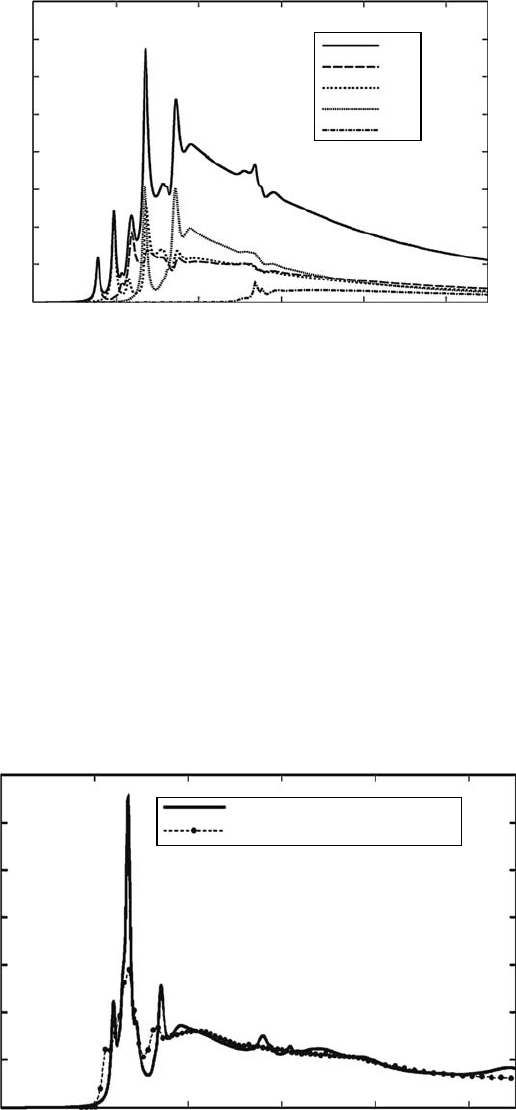
We show the TDDFT calculation for the oscillator strength distribution of H

O molecule below 55eV

in Figure 4.5, in comparison with measurement (Chan et al., 1993b). The decomposition of the strength

into occupied orbitals is shown in Figure 4.6 for the same energy region. The calculated energy of

HOMO orbital is 13.06eV, which is slightly larger than the measured ionization potential, 12.61eV. As

seen from Figure 4.5, the overall features of the oscillator strength distribution are well reproduced by

the calculation. The transition at around 8eV comes from the 1b

orbital. The next one around 10eV

is 3a

. These two transitions are visible in the measurement. In the calculation, next transition appears

around 11eV, which is from 1b

. The large transition at around 12eV, which is visible in the measure-

ment, comes from two orbitals, 3a

and 1b

. In the calculation, a Fano-like structure is seen at around

0.5

0.4

Total

1π

3σ

2σ

0.3

0.2

0.1

5 10 15

Oscillator strength distribution (eV

–1

)

Energy (eV)

20 25 30

Figure 4.4 Decomposition of the calculated oscillator strength distribution of O

molecule into orbitals.

0.4

0.35

0.3

0.25

0.2

0.15

0.1

Cal.

Exp. (Chem. Phys. 178 (1993) 387)

0.05

0 10 20 30

Energy (eV)

Oscillator strength distribution (eV

–1

)

40 50

Figure 4.5 Oscillator strength distribution of H

O molecule. Calculation by TDDFT is compared with

measurement.

(Data from Chan, W.F. et al., Chem. Phys., 178, 38, 1993b.)

78 Charged Particle and Photon Interactions with Matter

28eV, which comes from 2a

orbital and is close to the threshold of 2a

orbital whose orbital energy is

30.08eV. In the measurement, such feature is not visible.

For the H

O molecule, Dupin et al. (2002) made a calculation employing the Stieltjes moment

method.

Cacelli et al. (1991) made a calculation with the K-matrix method.

4.4.1.4 C

molecule

We show the TDDFT calculation for the oscillator strength distribution of CO

molecule below

55eV in Figure 4.7, in comparison with measurement (Chan et al., 1993c). The decomposition of the

strength into occupied orbitals is shown in Figure 4.8 for the same energy region. The calculated

energy of HOMO orbital is 14.96eV, which is slightly larger than the measured ionization poten-

tial 13.78eV. As seen from Figure 4.7, the overall features of the oscillator strength distribution

are again well reproduced by the calculation. The transition at around 12eV is composed of several

transitions. At least four transitions are seen in the calculation that originate from 1π

, 1π

, 3σ

, and 4σ

0.4

0.35

0.3

0.25

0.2

0.15

0.1

0.05

0 10 20 30

Energy (eV)

Oscillator strength distribution (eV

–1

)

40 50

Total

Figure 4.6 Decomposition of the calculated oscillator strength distribution of H

O molecule into orbitals.

1.4

1.2

0.8

0.6

0.4

Cal.

Exp. (Chem. Phys. 178 (1993) 401)

0.2

0 10 20 30

Energy (eV)

Oscillator strength distribution (eV

–1

)

40 50

Figure 4.7 Oscillator strength distribution of CO

molecule. Calculation by TDDFT is compared with

measurement.

(Data from Chan, W.F. et al., Chem. Phys., 178, 401, 1993c.)

Time-Dependent Density-Functional Theory for Oscillator Strength Distribution 79

Thenext one around 17 eV comes from 1π

and 3σ

orbitals. In the calculation, there appear a few

transitions around 30eV, which is originated from the 2σ

orbital whose orbital energy is 33eV.

However,

they are not visible in the measured spectrum.

For

the CO

molecule, Olalla and Martin (2004) made a calculation with the molecular quantum

defect

orbital method.

4.4.2 hydrocarbon MoleculeS

We report the oscillator strength distributions of several hydrocarbon molecules of small and

medium sizes. In addition to molecules shown below, we reported the oscillator strength distribu-

tions

of C

isomers in (Nakatsukasa and Yabana, 2004).

4.4.2.1 acetylene

We show the TDDFT calculation for the oscillator strength distribution of the acetylene, C

molecule below 40eV in Figure 4.9, in comparison with measurement (Ukai et al. 1991, Cooper et al.

1.4

1.2

0.8

0.6

0.4

Total

1π

3σ

4σ

2σ

3σ

0.2

0 10 20 30

Energy (eV)

Oscillator strength distribution (eV

–1

)

40 50

Figure 4.8 Decomposition of the calculated oscillator strength distribution of CO

molecule into orbitals.

0.8

0.6

0.4

0.2

0 5 10 15 20

Energy (eV)

Oscillator strength distribution (eV

–1

)

Cal.

(e,e) exp.

Photon exp.

30 35 40

Figure 4.9 Oscillator strength distribution of acetylene, C

, molecule. Calculation by TDDFT is com-

pared with measurement. (Data from Ukai, M. et al. J. Chem. Phys., 95, 4142, 1991; Cooper, G. et al., J. Electron

Spectrosc. Relat. Phenom., 73, 139, 1995b.)