Hammond C. The Basics of Crystallography and Diffraction
Подождите немного. Документ загружается.


314 The stereographic projection and its uses
(or petrofabric diagram
2
) showing the orientations of the c-axes of the quartz grains in
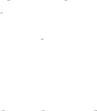
a metamorphosed psammite rock. They lie, as can be seen, roughly in a great circle,
the zone axis of which is closely parallel to the direction of lineation or structural long
direction of the rock.
Exercises
12.1 Prove that the stereographic projection of a small circle on the stereographic sphere is again
a circle. (Hint: this is an exercise in Euclidean geometry.)
12.2 Use the Wulff net to prepare a projection of a cubic crystal with (001) in the centre as in
Fig. 12.6. Find, by drawing in additional great circles, the positions of the (212) and (
¯
3
¯
32)
planes, measure their angles α, β and γ to the x, y and z axes and hence check that the
ratios of their direction cosines cos α: cos β: cos γ are in the ratios of h : k : l in each case
(see Section 5.5).
12.3 Two planes in a cubic crystal make the following angles to the crystal axes
x-axis y-axis z-axis
Plane A +36.5
◦
+57.5
◦
+74.5
◦
Plane B −48.2
◦
−70.5
◦
+48.2
◦
Find the positions of these planes on a standard projection from the common intersections
of small circles centred about the x, y and z-axes, and determine their Miller indices. Using
the Wulff net measure the angles between: PlaneA and Plane B; Plane A and (
¯
1
¯
11); Plane B
and (101); Plane Band (
¯
101).
12.4 Using sketch stereograms as in Fig. 12.12, show that (a)
¯
2 ≡ a perpendicular mirror plane;
(b)
¯
3 ≡ 3 +a centre of symmetry, and (c)
¯
6 ≡ 3 +a perpendicular mirror plane.
2
Petrofabric (or fabric) diagrams may also be represented on equal area projections which are, of course,
much used in earth science and geography since they show, for example, the sizes of materials in their correct
proportions. ‘Equal area graph paper’ consists, like the Wulff net, of intersecting small and great circles, but
these are not arcs of circles and do not appear to intersect at 90
◦
. The geometry of equal-area projection is
more complicated than that of the stereographic projection. For example, referring to Fig. 12.2, we need to
project the points on the sphere 15
◦
,30
◦
, etc. from the north pole such that they make equal divisions along
the equatorial plane, and this cannot be done by projecting lines down to a single point.

13
Fourier analysis in diffraction and
image formation
13.1 Introduction—Fourier series and Fourier transforms
In many areas of physics we encounter physical events, characteristics or properties
which repeat at regular intervals and which may be represented by waveforms of var-
ious shapes and complexity. Perhaps the most familiar examples are the sound waves
produced by musical instruments, where the waveforms represent air pressure variations
and the repeat distance or wavelength represents the frequency or pitch of the funda-
mental note. Figure 13.1 shows three such waveforms; the characteristic ‘sound’of each
instrument is related to the shape of the waveform in each case. Another example is a
simple diffraction grating which has a waveform consisting of flat-topped peaks (corre-
sponding to the light from the slits) with dark regions in between (Fig. 13.7(a) below).
Such waveforms are called periodic functions and are also of great importance in crys-
tallography because, as we shall see below, crystal structures can be represented in terms
of periodic variations of electron density, the density peaking at the atom positions and
falling to low values in between.
Flute
Oboe
Violin
Fig. 13.1. Examples of waveforms of musical instruments (from Measured Tones by I. Johnston,
Adam Hilger (Institute of Physics), Bristol, 1989).
316 Fourier analysis in diffraction and image formation
Jean Baptiste Fourier
∗
showed that any periodic waveform or function could be
analysed in terms of a series of cosine or sine waveforms (or, more generally, a series
of exponential functions). First, a ‘constant’ term (representing, in sound waves, the
undisturbed air pressure or, in crystals, a uniform ‘sea’ of electrons); then a term with
a wavelength or repeat distance corresponding, in sound, to the fundamental note, or
in a crystal to the lattice repeat distance, then a term of half the wavelength (or twice
the frequency) corresponding, in sound, to the first harmonic, and so on. Each of these
cosine or sine waves is defined by its amplitude and phase—the phase representing the
displacements of the waves with respect to each other.
The process of analysing a complex waveform into a series of such components is
called Fourier analysis. Conversely, the generation of a complex waveform from such
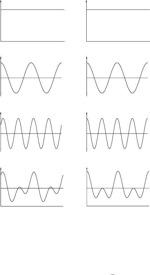
components is called Fourier synthesis. Figure 13.2 shows two examples in which the
complex waveforms (a) and (b) are synthesized from, or analysed into, three terms: a
constant term, a fundamental term and a first harmonic term. Notice that in (a) there is
a phase difference between the component waves which gives rise to the synthesized
asymmetrical waveform whereas in (b) there is zero (or a 180
◦
phase difference depend-
ing as to where you take the origin) which gives rise to the symmetrical waveform. In
crystallography (a) corresponds to electron density variations in a crystal without a centre
of symmetry whereas (b) corresponds to a crystal with a centre of symmetry (or a mirror
plane or diad axis normal to the direction in which the electron density is measured).
The amplitude A versusdistance x of aperiodicfunction is represented mathematically
by a Fourier series:
A = A
0
+ A
1
cos
2π1
x
a
− α
1
+ A
2
cos
2π2
x
a
− α
2
+···
+ A
n
cos
2πn
x
a
− α
n
i.e.
A =
n=N
n=0
A
n
cos
2πn
x
a
− α
n
where a is the repeat distance, the amplitudes A
1
, A
2
, ..., A
n
are called the Fourier coef-
ficients and α
1
, α
2
, ..., α
n
are the phase angles. The Fourier series may equally well be
written in terms of sines or, more generally, exponential terms, but in cases where the
waveform is symmetrical (as in crystals with a centre of symmetry or a simple diffraction
grating and in which the phase angles are zero or 180
◦
) we shall find the cosine form
more convenient: a cosine is a symmetrical function, i.e. cos x = cos(−x) whereas a
sine is an asymmetrical function, i.e. sin x =−sin(−x). Hence the Fourier series may
be written:
A = A
0
+ A
1
cos 2π1
x
a
+ A
2
cos 2π2
x
a
+···+A
n
cos 2πn
x
a
∗
Denotes biographical notes available in Appendix 3.
13.1 Introduction—Fourier series and Fourier transforms 317
0
0
0
0
(1)
Constant
term
(2)
Fundamental
term
(3)
First harmonic
term
Fourier
synthesis
of (1)+(2)+(3)
0
0
0
0
(a)
(b)
Fig. 13.2. Fourier synthesis of a complex waveform from three components: a constant term (1), a
fundamental term (2) and a first harmonic (3). The asymmetrical waveform in (a) arises from the phase
difference between the fundamental term and first harmonic. (Courtesy of Mr D.G. Wright.)
i.e.
A =
n=N
n=0
A
n
cos 2πn
x
a
.
The first term A
0
represents, in effect, a wave of infinite wavelength (in sound the
undisturbed air pressure), the second a wave of amplitude A
1
, and wavelength a (in
sound the fundamental note), the third a wave of amplitude A
2
and wavelength a/2 (in
sound the first harmonic), and so on. The Fourier coefficients A
0
, A
1
, A
2
, etc. may also
318 Fourier analysis in diffraction and image formation
be represented as components on a frequency scale A
0
(zero frequency), A
1
(frequency
2π/a), A
2
(frequency 4π/a), and so on.
Finally, there is a very important development in Fourier analysis (though not envis-
aged by Fourier himself) and that is that it can also be applied to non-periodic functions
such as a single sound pulse or the distribution of light from a single slit or aperture. This
may be donebyenvisaging a non-periodic function as, in effect, a periodic function with a
fundamental repeat distance that approaches infinity. In this case the Fourier coefficients,
represented as components on a frequency scale, approach closer and closer together
(the frequency differences become smaller and smaller) until they merge together. The
envelope of all the merged-together Fourier coefficients is called the Fourier transform
and is treated mathematically as an integral, rather than a summation of the Fourier
series for a periodic function. As we shall see, the diffraction pattern from a single slit or
aperture (expressed as an amplitude, rather than an intensity distribution) and the Fourier
transform are synonymous.
13.2 Fourier analysis in crystallography
In our derivation of the structure factor F
hkl
(Section 9.2), we considered the atoms to
be discrete scattering centres, the atoms being located at specific points in the unit cell
denoted, for the nth atom, by the fractional coordinates (x
n
y
n
z
n
). The atomic scattering
factor f
n
was derived by considering the interference of all the waves scattered by the
z electrons in the atom and then the structure factor F
hkl
was obtained by considering
the interference of all the scattered waves from all the atoms in the unit cell. Hence we
obtained the relation:
F
hkl
=
n=N
n=0
f
n
exp 2πi
(
hx
n
+ ky
n
+ lz
n
)
.
We are now going to determine F
hkl
starting, as it were, from a different standpoint. Since
it is the electrons which scatter X-rays then we are really detecting the distribution, or
variation in the ‘density’ of electrons throughout the unit cell, the electron density being
greatest at the atom centres and falling to low values in between. In short we have a
three-dimensional periodic variation in electron density, the variation being repeated (as
for the lattice) from cell to cell.
It is not easy to represent such electron density variations in three dimensions except
for the simplest crystals. It is much easier to represent the projection of electron density
on to one face of the cell—just as we represented crystal structures in terms of projections
or plans (Section 1.8). Figure 13.3 shows a ‘classic’ example: a projection on the (010)
face of the monoclinic mineral diopside, CaMg(SiO
3
)
2
. Figure 13.3(a) shows the atom
positions and Fig. 13.3(b) the corresponding electron density ‘contour map’—the peaks
corresponding to the heavy, overlapping Ca and Mg atoms and the diffuse ‘ridges’ in
between corresponding to the distribution of the lighter O and Si atoms.
We now need to replace the atomic scattering factor f
n
in the equation by an equivalent
electron-density term. Let ρ
xyz
be the electron density (number of electrons per unit vol-
ume) at distance coordinates xyz in the unit cell. We use these coordinates in preference
13.2 Fourier analysis in crystallography 319
c
a
Ca
O
2
Si
O
1
O
3
(a)
(b)
a
c
Volume element
edges dx, dy, dz
Mg
Fig. 13.3. (a) Projection of the atom positions in diopside, CaMg(SiO
3
)
2
, on to the (010) face and
(b) the corresponding electron density ‘contour map’. Also indicated is a volume element dV, at distance
coordinates xyz and edge-lengths dx, dy, dz. (Adapted from W.L. Bragg, Zeitschrift für Kristallographie
70, 475, 1929.)
to the fractional coordinates used in Chapter 9, i.e. x (fractional) = x (distance)/a and
similarly for y and z. Now we outline a small volume element with edges dx, dy, dz
parallel to the unit cell axes a, b, c as indicated in Fig. 13.3(b). Let dV be the volume
of this element and V the volume of the unit cell. The ratio dV /V equals the ratio
dxdydz/abc, whence dV =
V
abc
dxdydz (for orthogonal axes of course dV = dxdydz).
The number of electrons in the volume element is simply ρ
xyz
dV =
V
abc
ρ
xzy
dxdydz
which we now replace for f
n
in the structure factor equation. However, since ρ
xzy
is a
continuous function we must also replace the summation by a triple integral, i.e. along
all three axes. Hence the structure factor equation becomes:
F
hkl
=
V
abc
a
0
b
0
c
0
ρ
xyz
exp 2πi
h
x
a
+ k
y
b
+ l
z
c
dxdydz.
320 Fourier analysis in diffraction and image formation
x
r
x
dx
a = d
100
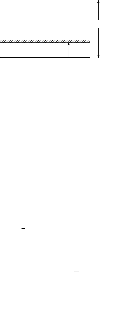
Fig. 13.4. Representation of electron density as a ‘slab’ of thickness dx parallel to one set of lattice
planes of spacing (repeat distance) a.
In order to proceed further with this equation we need to express the electron density ρ
xyz
in terms of a three-dimensional Fourier series. However, without loss of principle, we
shall carry out the analysis in one dimension (corresponding to reflections from one set of
crystal planes) and also for a crystal with a centre of symmetry in which the phase angles
of the Fourier components are all zero or 180
◦
(i.e. the signs of the Fourier coefficients
are all + or −).
Consider Bragg reflection from one set of lattice planes (100) with a spacing a (= d
100
for orthogonal axes), Fig. 13.4. As we know it is a consequence of Bragg’s law (Fig. 8.3)
that the interference conditions for the scattered waves are the same irrespective of the
positions of theatoms parallel to the planes. Referring to the simpleexample in Fig. 9.2(b)
the atom f
1
may be located anywhere along the dashed line: the phase angle φ
1
is solely
determined by the component of r
1
perpendicular to the planes. Hence (Fig. 13.4) we
can only specify the electron density, ρ
x
, in the x-direction and must therefore replace
the volume element with a ‘slab’ or ‘layer’ of thickness dx and nominal unit area. The
number of electrons in the slab is then simply ρ
x
dx.
We now express ρ
x
in terms of a one-dimensional Fourier series:
ρ
x
= A
0
+ A
1
cos 2π1
x
a
+ A
2
cos 2π2
x
a
+···+A
n
cos 2πn
x
a
ρ
x
=
n=N
n=0
A
n
cos 2πn
x
a
.
Now we writethe structure factor equation for F
h00
for a crystalwith a centre of symmetry
and also using distance coordinates instead of fractional coordinates:
F
h00
=
n=N
n=0
f
n
cos 2πh
x
n
a
.
Substituting f
n
by ρ
x
dx and replacing, as before, the summation by an integral (ρ
x
is a
continuous function) we have:
F
h00
=
x=a
x=0
ρ
x
cos 2πh
x
a
dx.
13.2 Fourier analysis in crystallography 321
Then, substituting for ρ
x
and interchanging the integral and summation signs we have:
F
h00
=
n=N
n=0
x=a
x=0
A
n
cos 2πn
x
a
cos 2πh
x
a
dx.
Now, remembering the trigonometrical identity:
cos A cos B =
1
2
[
cos
(
A + B
)
+ cos
(
A − B
)
]
we have:
F
h00
=
1
2
n=N
n=o
A
n
⎡
⎣
x=a
x=0
cos 2π
(
n + h
)
x
a
dx +
x=a
x=0
cos 2π
(
n − h
)
x
a
dx
⎤
⎦
.
Now, since n and h are integers the integrals express the total area for one complete cycle
of the cosine curve and are thus zero since the areas above and below zero cancel out
except for the cases where (n + h) and (n − h) are zero, in which case the integrals are
x=a
x=0
cos 0 dx = a.
Hence, the equation reduces as follows:
When h = n = 0; F
000
=
1
2
A
0
[
a + a
]
= A
0
a
When n = h; F
h00
=
1
2
A
h
[
0 + a
]
= A
h
a/2
When n =−h; F
¯
h00
=
1
2
A
¯
h
[
a + 0
]
= A
¯
h
a/2.
This isa profoundresult, firstenvisaged byW.H.Bragg in 1915. It showsthat each Fourier
coefficient is equal (apart from the scaling factor a) to the corresponding structure factor.
In the general case, where the structure factors are complex numbers, so also are the
Fourier coefficients and for reflections hkl the relations are written F
hkl
= VA
hkl
where
V is the volume of the unit cell.
We may now rewrite the Fourier series equation for ρ
x
substituting for A
0
=
(1/a)F
000
, A
h
= (2/a)F
h00
and A
¯
h
= (2/a)F
¯
h00
and summing for both positive and
negative values of h:
ρ
x
=
1
a
h=+N
h=−N
F
h00
cos 2πh
x
a
and for the general three-dimensional case:
ρ
xyz
=
1
V
N
h
k
l
−N
F
hkl
exp 2πi
h
x
a
+ k
y
b
+ l
z
c
.
322 Fourier analysis in diffraction and image formation
CI
CI
A
2
A
4
A
0
A
5
A
3
A
1
Na
r
Fig. 13.5. The variation in electron density ρ normal to the (111) planes in NaCl. On the left are shown
the Fourier componentsA
0
, ..., A
5
, each of which correspondto the structurefactors F
000
, F
111
, ..., F
555
.
(Adapted from X-ray Analysis of Crystals by J.M. Bijvoet, N.H. Kolkmeyer and C.H. MacGillavry,
Butterworths, London, 1951.)
Figure 13.5 shows a one-dimensional Fourier synthesis of the electron density perpen-
dicular to the (111) planes of NaCl which consist of alternate layers of Na and Cl atoms.
The electron density, which is symmetrical about both Na and Cl atoms, is the sum of
five components, A
0
, ..., A
5
with coefficients corresponding to F
000
,2F
111
, ...,2F
555
.
For h, k, l all even F
hkl
= 4
(
f
Cl
+ f
Na
)
and for h, k, l all odd F
hkl
= 4
(
f
Cl
− f
Na
)
.
Hence, using f vs. sin θ/λ data from the International Tables the F
hkl
values and hence
the values of the Fourier coefficients can be determined.
This of course is a simple case because all of the structure factors are real and positive
(origin at a Cl atom). Notice that the electron-density curve lies equally above, and
below, the A
0
term which represents a uniform ‘sea’ of electron density.
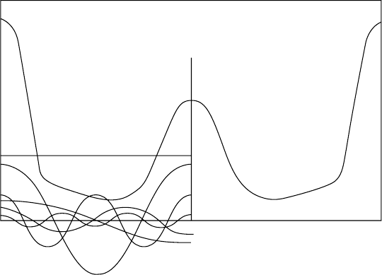
Hopefully, it is now easy to see how atoms are located at the intersecting maxima
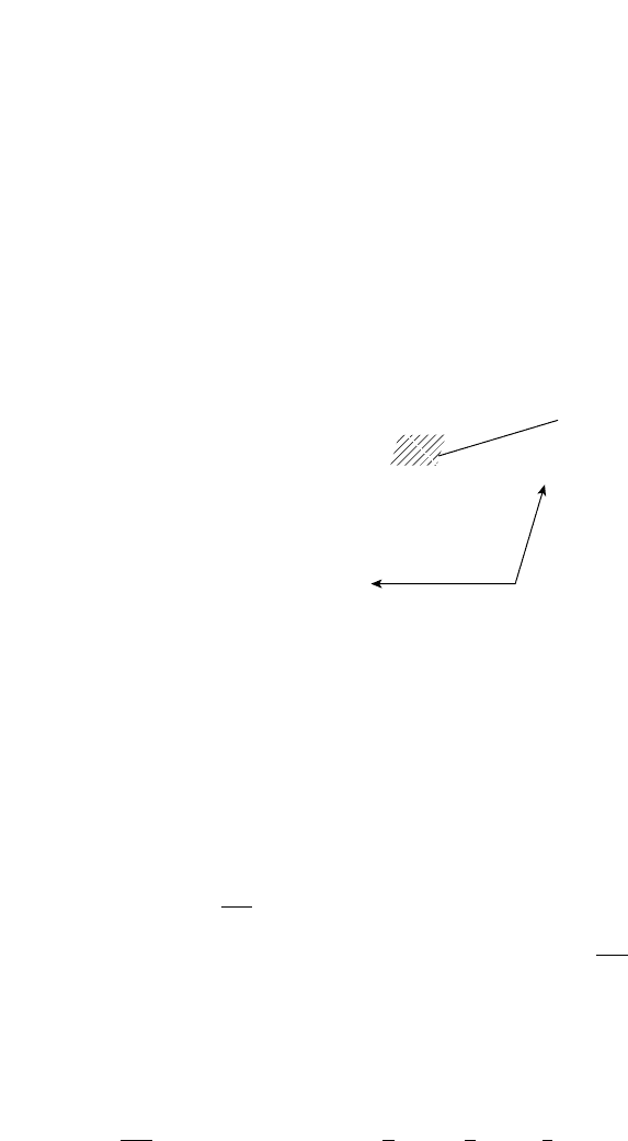
of electron density waves from different sets of reflections. Figure 13.6 shows just
two waves, F
020
cos 2π2(y/b) and F
300
cos 2π3(x/a) (where a and b are the cell edge
lengths) and (below) their sum and projection as a contour map. Even at this low level
of resolution the locations of the atom centres are evident.
For crystals without a centre of symmetry, in which the structure factors are complex
numbers and their relative phases are unknown, we need to make use of further math-
ematical tools, the principal of which is the Patterson function which does not specify
the location of atoms, but rather the distribution of vectors, representing the distances
between them. However, this topic, and the determination of crystal structures in general,
are beyond the scope of this book.

13.3 Analysis of the Fraunhofer diffraction pattern 323
F
020
cos 2 2 y/b
F
300
cos 2 3 x/a
Sum
Contour
map
Fig. 13.6. A two-dimensional contour map synthesized from just two Fourier components (upper
curves) and their sum (lower curve). Even at this low level of resolution the contour map shows discrete
maxima (from X-ray Crystal Structure by D. McLachlan, McGraw-Hill Book Company, 1957.)
13.3 Analysis of the Fraunhofer diffraction pattern
from a grating
Figure 13.7(a) shows the ‘square top’ waveform representing the amplitude of light
emerging from a grating consisting of six slits (N = 6), width d and spacing a, illu-
minated by an incident plane wave normal to the grating. Figure 13.7(b) shows the
corresponding diffraction pattern. First, we recapitulate the simple analysis given in
Section 7.4.
(1) The envelope of the pattern (dashed curve) corresponds to the intensity profile for a
single slit with minima at sin α angles 1
λ
d
,2
λ
d
,3
λ
d
, etc.
(2) The principal maxima correspond to the conditions for constructive interference
between the slits at sin α angles 1
λ
a
,2
λ
a
,3
λ
a
, etc.
(3) The minima of the subsidiary maxima correspond to the conditions for destructive
interference for the whole grating considered as a single slit of width 6a, i.e. at sin α
angles 1
λ
6a
,2
λ
6a
,3
λ
6a
, etc.