Gulian A.M., Zharkov G.F. Nonequilibrium Electrons and Phonons in Superconductors

Подождите немного. Документ загружается.

SECTION 11.3. FINITE TEMPERATURES 301

11.3.2. -Approximation

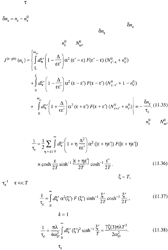
The deviation of the electron distribution function from its equilibrium value

is assumed to be small and localized in an energy range much smaller

than the temperature scale. In such a case, the terms containing in the integrands

are small compared with the terms containing as multipliers. Omitting these

integral terms and noting that the terms in square brackets in Eq. (11.34) vanish for

the equilibrium substitutions and one can write:

After algebraic manipulations, taking into account the expressions for and

one finds

Because the essential range of integration in (11.36) is one can consider

at as a constant:

which in the Debye model [ in (11.2)] is equivalent to

Note that this expression for , as well as the collision integral in the relaxation-time

approximation, was used in previous chapters.

302 CHAPTER 11. INFLUENCE OF LASER RADIATION

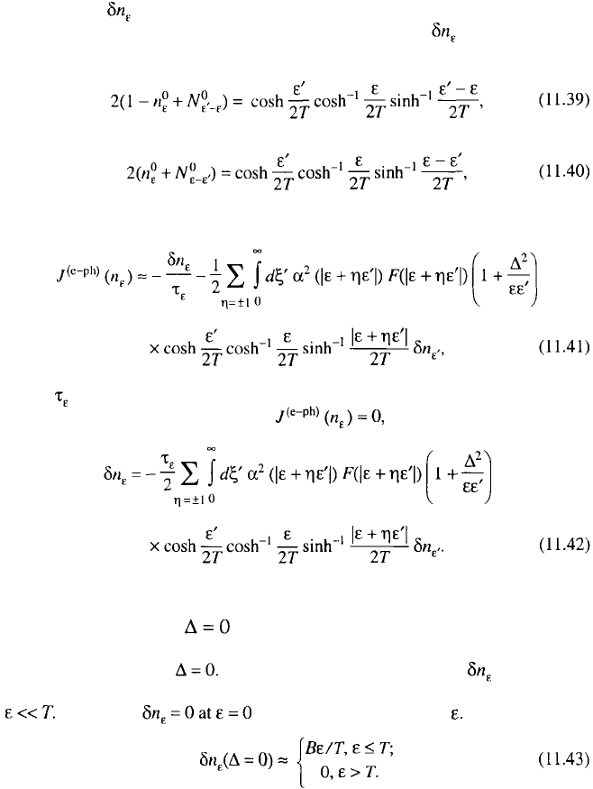
11.3.3. Iterative Solution Procedure

Continue now the examination of the collision operator (11.34), removing the

restriction for to be localized, but assuming it is small in magnitude. The only

simplification now follows from neglecting the quadratic in terms. Taking into

account the identities

one can rewrite (11.34) in the form:

where is given by Eq. (11.37). As in Sect. 11.1, the shape of the distribution

function is governed by the condition which implies:

11.3.4. Solution for

Let us initially put Then from (11.42) it follows that varies within

the energy range of the order of the temperature scale, decaying exponentially at

In our case and increases linearly with So:

The coefficient B may be estimated from the normalization condition, which is

analogous to (11.3):

SECTION 11.3. FINITE TEMPERATURES 303

Using the approximation (11.2) with one finds (by the order of magnitude)

11.3.5. Coherent Contribution

To estimate the contribution proportional to one can use an iteration

procedure based on (11.42). Substituting (11.43) into (11.42) and taking into

account (11.2) and (11.37), one can find the desired correction (up to the factor

cf.

Ref.

3):

In deriving Eq. (11.46) it was taken into account that the “coherent” correction

should be essential in the energy range The part of which does not

depend on was omitted, although it renormalizes the function

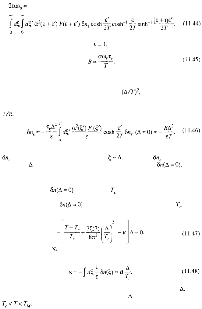
11.3.6. Two Branches of a Nonzero-Order Parameter

This function renormalizes in the self-consistency equation

(5.25). One can assume that this renormalization has been made and ignore the

explicit dependence on in Eq. (5.25), which in the vicinity of has the

form[cf. Eq. (1.182)]:

The anomalous part which sometimes is called the gap control term (see Sect.

7.1.7), is defined by the relation

Note that the function (11.46) is negative and this enhances the value of For a

given B

one has two branches of solution for in the temperature range

304

CHAPTER 11. INFLUENCE OF LASER RADIATION

The quantity is defined by the relation Apart from

these solutions, there is also a trivial solution, Thus the situation at finite

temperatures is analogous to the zero temperature case. In the next section we will

consider in more detail some consequences of this ambiguous behavior of the

nonequilibrium gap

11.4.

DISSIPATIVE PHASE TRANSITION

11.4.1. Stationary Solutions for Time-Dependent Problems

We will use in our analysis the time-dependent Ginzburg–Landau equation

(7.115) for a real order parameter, adding to (7.115) the contribution from the gap

control term caused by the action of an electromagnetic field:

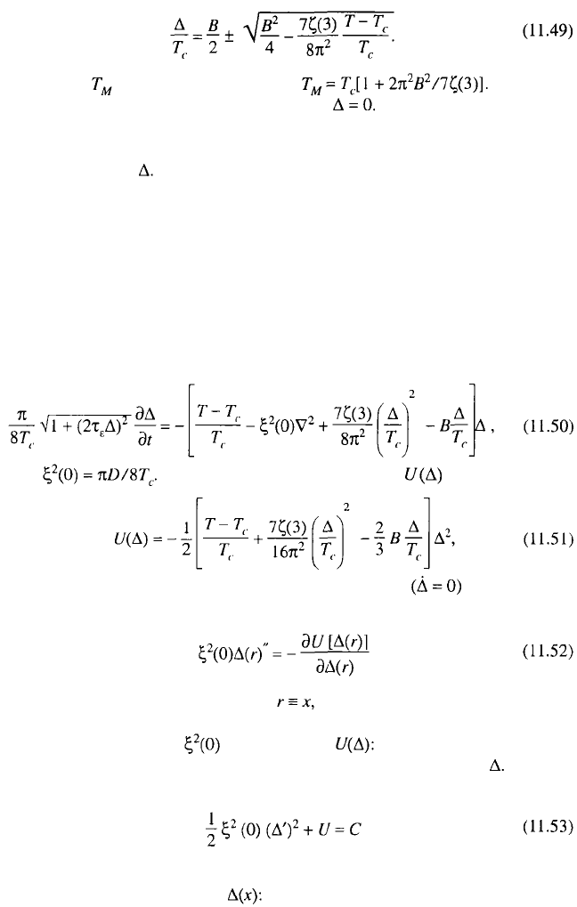
where Introducing the potential function

one finds from Eq. (11.50) that the stationary solutions must obey the

equation

(we consider the one-dimensional case omitting below the argument r

)

. As

was pointed out in Ref. 3, this equation is analogous to that describing the motion

of a particle with the mass in the potential instead of time we have the

space coordinate x, and instead of a space coordinate, the value of The first

integral of (11.52) has the form:

(the “mechanical” analogy to the constant C is the energy of the system). Note the

following properties of solutions the symmetry with respect to the coordinate

SECTION 11.4. DISSIPATIVE PHASE TRANSITION 305

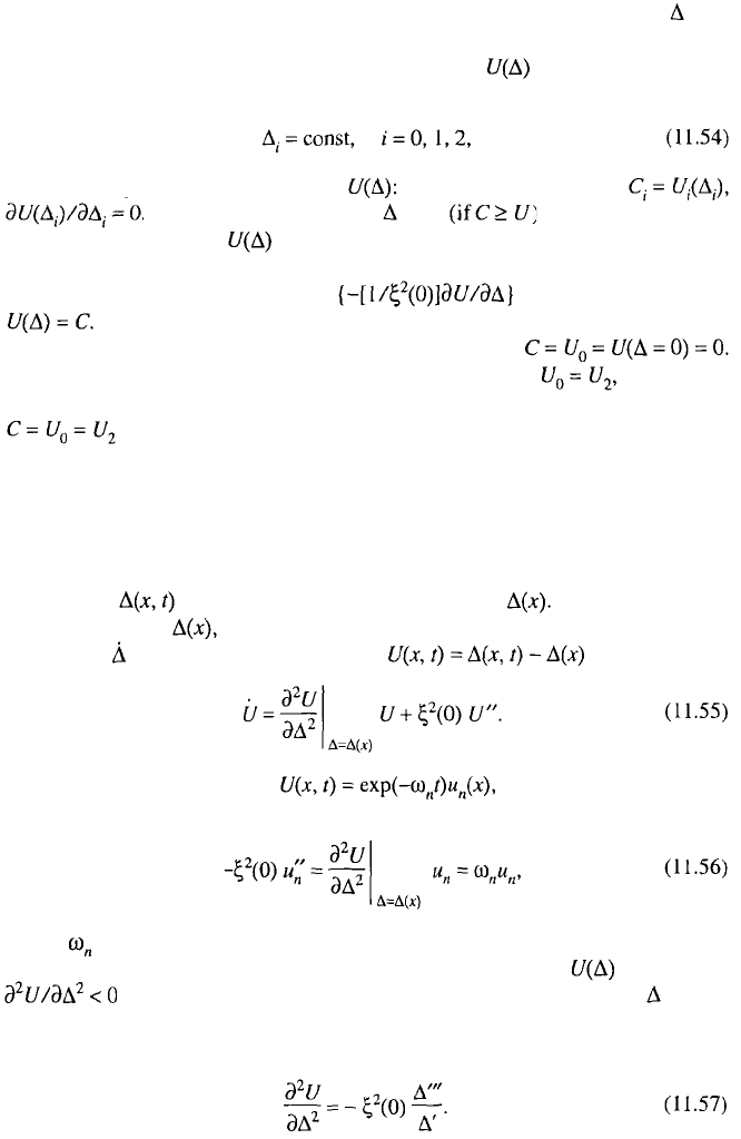
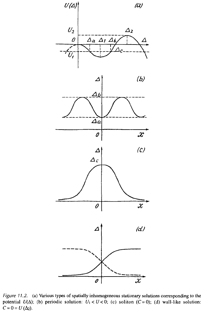
Among the solutions generated by the potential (Fig. 11.2a) there are

three constants:

which correspond to the extrema of in these cases we have

The restricted solutions for exist in the region between

the boundary extrema of (Fig. 11.2a). Generally these bounded solutions are

periodic in space (Fig. 11.2c). As follows from (11.52), the curvature in the extrema

of periodic solutions is equal to at the turning points

The periodic solutions degenerate to solitons (localized objects, Fig.

11.2c) whenever one of these curvatures vanishes, e.g., if

If for some reasons (e.g., at some level of external pumping) then there is

a possibility of further degeneration of the soliton to the wall-like solution at

(Fig. 11.2d).

11.4.2. Local Stability Against Space-Time Fluctuations

Now we will inspect, following Eckern et al.,

the local stability of these

solutions against small space–time fluctuations. To do this we will analyze the

dynamics of in the vicinity of stationary solutions Linearizing (11.50)

in the vicinity of and assuming (without any loss of generality) that the

prefactor at is equal to 1, one obtains for the equation:

Presenting U(x, t) in the form one obtains from (11.55)

the one-dimensional analogy of the “Schrödinger” equation:

where has the meaning of an “energy.” As follows from (11.56), spatially

homogeneous solutions corresponding to the maxima of are stable:

at these points. On the contrary, the intermediate values of are not

stable. To analyze the stability of spatially periodic stationary solutions, one should

differentiate (11.52), resulting in:

reflection and the invariance at an arbitrary shift of the “coordinate” (the

mechanical analogy is the time reversal and space translation).

306

CHAPTER 11. INFLUENCE OF LASER RADIATION

SECTION 11.4. DISSIPATIVE PHASE TRANSITION 307

Using (11.56) and (11.57), one can establish that the eigenfunction is the

only one that corresponds to the eigenvalue For periodic solutions,

has an infinite number of nodes. Hence there are functions with a finite number of

nodes that correspond to the lower values of “energy”: So the periodic

solutions are not stable. The soliton function has a single node; consequently

there is one eigenfunction corresponding to the smaller value of “energy”:

(the “ground state”). Thus the solitons are not stable either. The wall-like

solution has no nodes; this solution is stable against small perturbations.

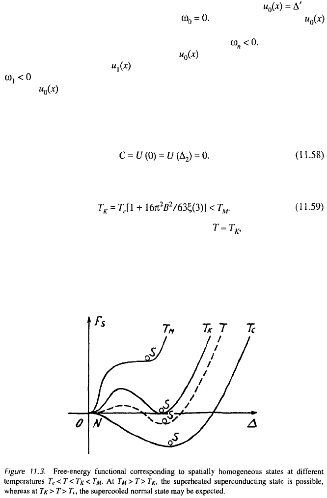
11.4.3. Coexistence of Normal and Superconducting States

As mentioned earlier, the wall-like solution corresponds to

Taking into account (11.51), it can be found from Eq. (11.58) that the wall-like

solution corresponds to the temperature

The general situation is illustrated in Fig. 11.3. At the free energies of

superconducting and normal phases are equal: these phases may coexist. At higher

temperatures, the normal phase is energetically favorable and the wall moves

toward the superconducting region. At lower temperatures, the superconducting

state is more favorable and the superconducting phase should expand to fill the

space.

308 CHAPTER 11. INFLUENCE OF LASER RADIATION

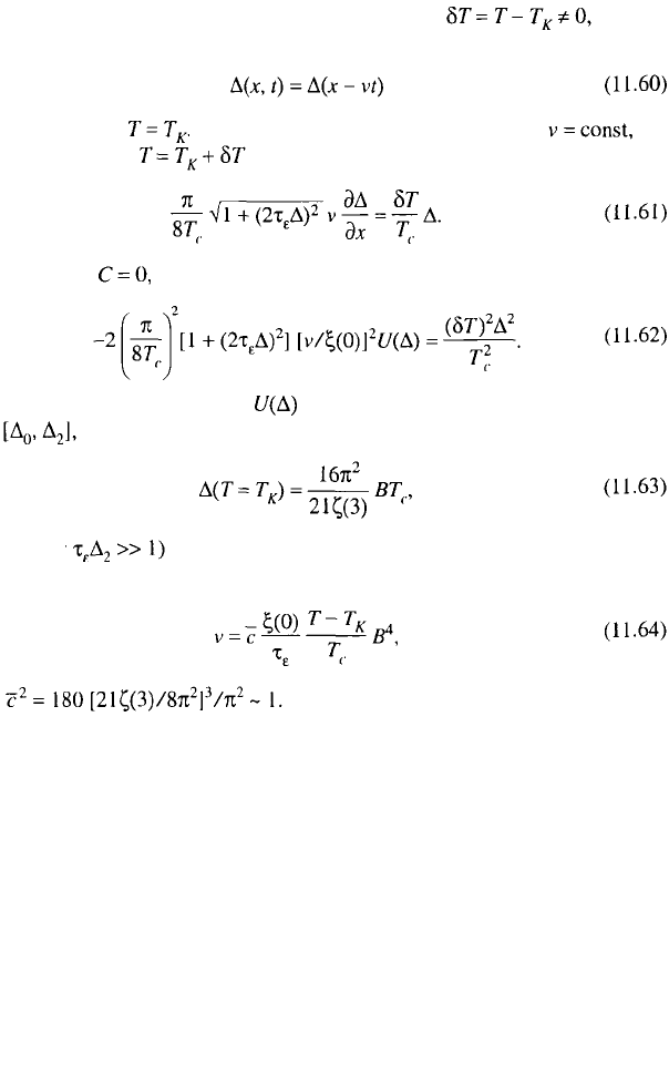
11.4.4. Velocity of Phase-Boundary Motion

To obtain the velocity

of NS boundary motion at one can

use (cf. Ref. 4) Eq. (11.50). Suppose the motion is stationary and the solution

obeys Eq. (11.52) at On account of (11.60) and the condition Eq.

(11.50) transforms at into

Using (11.53) at one obtains

Integrating expression (11.51) for along the trajectory of motion within the

limits taking into account Eq. (11.59) and

one finds (for the following expression for the motion of the wall (i.e.,

the NS boundary):

where

Because the spatially homogeneous solutions are locally stable, superheated

and supercooled states are possible. The transitions between different phases should

be analogous to the first-order phase transitions. The dynamics of these dissipative

phase transitions were discussed earlier.

11.5. MAGNETIC PROPERTIES

11.5.1. Equilibrium Diamagnetic Response

The response of a superconductor to a slowly varying magnetic field is

determined by the dependence of the superconducting current on the vector

potential. This dependence is contained in the first term of Eq. (7.88) (

= 1):

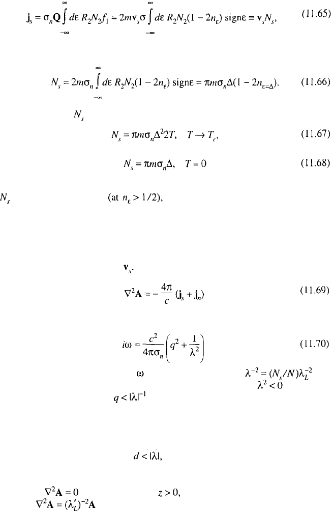
SECTION 11.5. MAGNETIC PROPERTIES 309

where

Positive values of in thermodynamic equilibrium

lead to a diamagnetic response. In a nonequilibrium state, as follows from (11.66),

may become negative which corresponds to the paramagnetic

response.

11.5.2.

Paramagnetic Instability

The superconducting paramagnetic state may become unstable against fluc-

tuations of superfluid velocity

5, 6

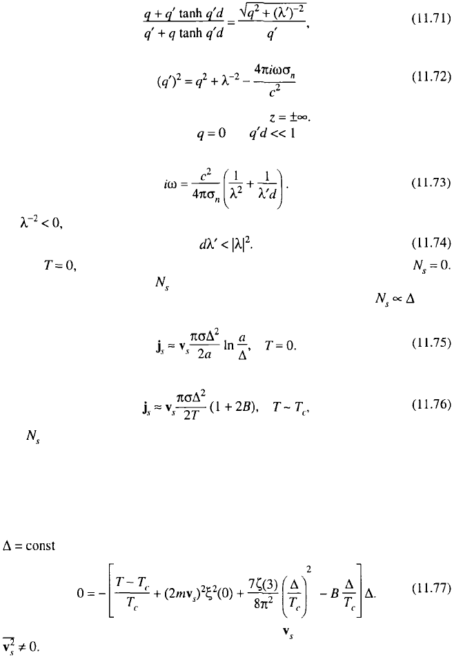
Indeed, from the Maxwell equation

the dispersion relation

follows for small values of q and subject to (11.65). Here and

N is the charge carrier density in the normal metal. Evidently for the Fourier

component of the field with grows exponentially in time.

11.5.3.

Role of Boundary Conditions

Thus the perturbations moving perpendicular to the boundary would be

damped out in a film of thickness while the perturbations moving along the

film would amplify. Note that such amplification may not occur if the film is

deposited on a massive superconductor S´.

In this case, one must consider three

equations: for the half-space Eq. (11.69) for the film S, and the

equation for the half-space occupied by a superconductor S´. These

310 CHAPTER 11. INFLUENCE OF LASER RADIATION

equations are linked by the boundary conditions expressing the continuity of the

vector potential

. The dispersion relations

follow for the solution, which should vanish at Because small values of

momenta are of interest, one can put and , obtaining thus from (11.71)

and (11.72):

At the system is stable if

If the substitution of (11.14) into (11.66) gives the value

Consequently, the sign of is defined mainly by the sign of the “coherent”

addition. As follows from (11.18), in the case we have considered, and is

positive. Using (11.8), (11.14), (11.65), and (11.66), one finds

In the model considered in Sect. 11.4, at finite temperatures one has

i.e., is also positive.

11.5.4. Superheated States at External Pumping

Concluding this section, we will discuss some peculiarities of the dissipative

phase transition in a magnetic field.

3,8,9

Suppose a thin film of thickness d (under

the action of laser radiation) is placed in a magnetic field H. In this stationary state,

and Eq. (11.65) is modified to

It was shown in Sect. 1.2 that the average value of in the film is zero, although

It could be evaluated as