Gubbins D., Herrero-Bervera E. Encyclopedia of Geomagnetism and Paleomagnetism

Подождите немного. Документ загружается.

(Cushman-Roisin, 1994). In rotating, electrically conducting fluids,

Lorentz force-driven shear flows are sometimes called magnetic winds.

Thermal wind in the core

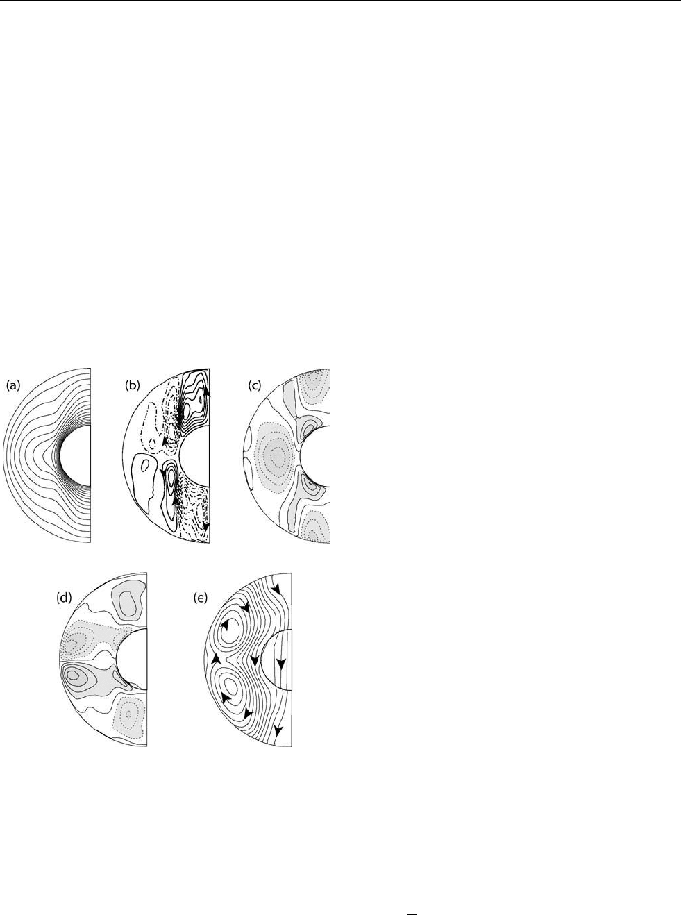
The general pattern of zonal flow we expect in the outer core is illu-

strated in Figure T3, which shows cross sections of the time-averaged

zonal temperature, fluid motion, and magnetic field structure from a

numerical dynamo model. This dynamo is driven by thermal convec-

tion and the lateral density variations are proportional to the lateral

temperature variations. The model is a highly idealized (and probably

over-simplified) representation of the geodynamo, but it illustrates the

basic structure of thermal winds in a rotating, convecting dynamo.

Although some of the input parameters are not accurately scaled (in

particular, the rate of rotation is far too slow for the Earth and the fluid

has higher electrical conductivity than the outer core) the model gives

realistic results for several important properties. For example, its exter-

nal magnetic field is dipole-dominant, like the geomagnetic field, and

it tends toward axial symmetry when averaged over long periods of

time. At any instant, however, both the flow and the magnetic field

are not as symmetric, as shown in Figure T3. The magnetic secular

variation in this model exhibits a preference for westward drift,

especially near the poles, which is also Earth-like. These general

similarities with observed geomagnetic field behavior result from

fundamental constraints on convection in a rotating spherical shell,

and are not particular to this model. It is therefore reasonable to

assume that the pattern of zonal flow in the model may approximate

the time-averaged pattern of zonal flow within the Earth’s core.

The large amount of axial shear in Figure T3c and its spatial rela-

tionship to the lateral temperature variations in Figure T3a and the

meridional circulation in Figure T3b indicate the time-averaged zonal

velocity is mostly thermal wind. In contrast, there is very little colum-

nar motion in the time-averaged flow in this dynamo. In the Earth’s

core, there is evidence from the geomagnetic secular variation for

time-varying zonal columnar flow with periodicity of order one cen-

tury. Oscillating columnar core flow is thought to be important in the

exchange of momentum between the core and the mantle associated

with decade time-scale fluctuations in the length of the day. But the

existence of columnar flow in the core over longer periods of time

has yet to be established.

The time-average zonal temperature shows a basic octupole pattern.

Elevated temperatures occur near the equatorial plane in Figure T3a,a

consequence of efficient heat transport by small-scale convection,

which is suppressed by the zonal averaging and is not evident in the

velocity fields in Figure T3b and T3c. The thermal wind is particularly

strong within the axial cylinder containing the inner core, the inner

core tangent cylinder (q.v.). Here it is closely related to the axisym-

metric meridional circulation, which consists of a polar plume with

return flow along the tangent cylinder. Zonal flow inside the tangent

cylinder is directed westward near the core-mantle boundary, but

reverses direction with depth and becomes eastward near the inner

core boundary. The high-latitude westward motion near the core-

mantle boundary in both hemispheres are polar vortices, analogs to the

ozone-trapping polar vortices in the stratosphere. The eastward motion

of the thermal wind deep in the outer core results in viscous and elec-

tromagnetic stresses on the inner core boundary. The drag produced by

these stresses tends to make the inner core super-rotate, that is, spin

slightly faster than the mantle. This offers an explanation for the anom-

alous rotation of the inner core inferred by some seismic studies.

Figure T3c shows that the belts of eastward motion responsible for inner

core super-rotation extend out to the core-mantle boundary at midlati-

tudes. At lower latitudes, the thermal wind flow immediately below

the core-mantle boundary is weak, but at greater depth there is a sub-

merged westward jet centered on the equator, an equatorial undercurrent.

The combination of the westward undercurrent and the eastward

flow near the inner core boundary generates much of the toroidal com-

ponent of the magnetic field shown in Figure T3d. The shear contained

in these flows stretches the poloidal magnetic field lines shown in

Figure T3e, winding them into pairs of toroidal field coils with oppo-

site polarity in each hemisphere. This is an example of toroidal field

induction by the so-called o-dynamo effect, and is considered to be

a critical part of the geodynamo process in the core. The thermal wind

also influences the poloidal magnetic field, although in a different way.

Comparison of Figure T3e and T3c shows that the poloidal field lines

tend to align with the contours of the thermal wind velocity, a config-

uration that allows the field to nearly co-rotate with the thermal wind.

The tendency of poloidal field lines to align with the thermal wind is

an example of Ferraro’s (1937) law of co-rotation, a general magneto-

hydrodynamic principle that has been used to infer planetary rotation

rates from magnetic variations.

In rotating fluids where the lateral density variations are produced

by convection, the amplitude of the thermal wind obeys the following

relationship:

U 



1=2

;

where U is the r.m.s. thermal wind amplitude and F is the flux of

buoyancy associated with the convection. The same formula has been

Figure T3 Cross-sections of time- and azimuthally averaged

structure of a numerical dynamo model driven by thermal

convection in a rotating, electrically conducting spherical fluid

shell. The parameters of this model are the same as the thermal

convection benchmark dynamo of Christensen et al. (2001),

but with twice the rotation and heating rates. (a) Contours of

temperature; (b) streamlines of meridional circulation with flow

direction arrows; (c) contours of zonal velocity showing the

thermal wind; (d) contours of toroidal magnetic field intensity;

(e) poloidal magnetic field lines with direction arrows. Contour

shading is proportional to magnitude; solid and dashed lines

indicate positive and negative values, respectively. Zonal velocity

and toroidal magnetic field intensity are positive eastward.

Magnetic polarity in this model is normal relative to present-day

geomagnetic polarity; this has no effect on the flow.

946 THERMAL WIND

found to hold in convection-driven dynamos with relatively strong

magnetic fields, another consequence of Ferraro’s law of corotation

(Aubert, 2005). According to this relationship, a thermal wind velocity

of U ¼ 10

3

1

in the core, which is consistent with the observed

geomagnetic secular variation, is associated with a convective buoy-

ancy flux of about F ¼ 7  10

11

3

. This is within the range of

the buoyancy flux estimates based on the core’s present-day energy

budget (Aurnou et al., 2003). A scaling analysis of the thermal wind

equation reveals that the lateral density variations needed to maintain

a thermal wind flow with this amplitude in the core are less than one

part in a million (Jackson and Bloxham, 1991), too small, unfortu-

nately, to be observed in the gravity field or by seismic methods.

The high degree of symmetry in Figure T3 is a consequence of time

and azimuthal averaging. Significant departures from axial symmetry

are present in the thermal wind and the other variables at any instant,

because of transient chaotic fluctuations in the model. In the core,

similar transient chaotic fluctuations are also likely, and these might

account for the hemispheric asymmetry observed in the geomagnetic

field during historical times, and may be the cause of dipole excursions

and polarity reversals. Even longer-lasting deviations from symmetry

are also possible in the geodynamo, due to interaction of core flow

with heterogeneity in the lower mantle. It is well established that spa-

tial heterogeneity in boundary heat flow can produce localized thermal

winds in a rotating fluid (Sumita and Olson, 1999), and it has been

proposed that thermal winds in the core are tied to lower mantle het-

erogeneity by this mechanism. It has also been proposed that slow

changes in the core flow, responding to changes in the structure of

the lower mantle heterogeneity, can causes the long-term variations

observed in magnetic reversal frequency record (Gubbins, 1987).

In summary, multiple lines of evidence indicate thermal winds are

present in the core and affect the geodynamo in a variety of ways.

Much remains to be learned about the nature of these flows and their

relationship to the other parts of the Earth.

Peter Olson

Bibliography

Aubert, J., 2005. Steady zonal flows in spherical shell dynamos. Jour-

nal of Fluid Mechanics, 542:53–67.

Aurnou, J., Andreadis, S., Zhu, L., and Olson, P., 2003. Experiments

on convection in Earth’s core tangent cylinder. Earth and Plane-

tary Science Letters, 212:119–134.

Christensen, U.R., et al., 2001. A numerical dynamo benchmark. Phy-

sics of Earth and Planetary Interiors, 128:51–65.

Cushman-Roisin, B., 1994. Introduction to Geophysical Fluid

Dynamics. Englewood Clifts, NJ: Prentice-Hall.

Davidson, P.A., 2001. An Introduction to Magnetohydrodynamics.

New York: Cambridge University Press.

Ferraro, V.C.A., 1937. The non-uniform rotation of the sun and its

magnetic field. Monthly Notices of the Royal Astronomical Society,

97: 458.

Gubbins, D., 1987. Mechanism for geomagnetic polarity reversals.

Nature, 326: 167–169.

Jackson, A., and Bloxham, J., 1991. Mapping the fluid flow and

shear near the core surface using the radial and horizontal compo-

nents of the magnetic field. Geophysical Journal International,

105: 199–212.

Sumita, I., and Olson, P., 1999. A laboratory model for convection in

Earth’s core driven by a thermally heterogeneous mantle. Science,

286: 1547–1549.

Cross-references

Convection, Chemical

Core Convection

Core Motions

Dynamos, Mean Field

Geodynamo, Numerical Simulations

Inner Core Rotation

Inner Core Tangent Cylinder

Proudman-Taylor Theorem

TIME-AVERAGED PALEOMAGNETIC FIELD

The geocentric axial dipole hypothesis (q.v.), or GAD, is a central

tenet of paleomagnetism: the geomagnetic field is assumed to average

over time to a simple dipolar form aligned with the Earth’s rotation

axis. This enables measurement of past plate motion, continental drift,

and regional geological deformation. The dipole assumption allows

any magnetic direction determined at a site to be transformed to a vir-

tual geomagnetic pole (VGP), defining the axis of the assumed dipole.

Many VGPs determined within a single rock unit are found to cluster

about a center, called the paleomagnetic pole. The paleomagnetic pole

is treated as an estimate of the location of the geographic pole at the

time of formation of the rock unit; the scatter of VGPs is supposed

to be caused by geomagnetic secular variation. The latitude of the rock

unit at the time of its formation, and the angle through which the

rock unit has rotated since its formation, can be obtained from the

paleomagnetic pole position. The scatter of VGPs around the paleo-

magnetic pole provides an estimate of the error on the paleomagnetic

pole and hence the errors on the latitude and rotation of the rock unit.

Merrill and McElhinny (1996) discuss the establishment of the

GAD in detail. Simple clustering of the VGPs is not enough to demon-

strate dipolar structure: a definitive determination requires similar

paleomagnetic pole positions for a range of contemporary locations.

This is possible in the recent geological past when plate motions are

negligible or are well determined by other means; for the more distant

past it is possible to compare latitudes determined paleomagnetically

with those determined by paleoclimate. Statistical distributions of

paleomagnetic inclination can also be used to establish the dipole

structure. Adequate time sampling of the rock unit is also essential

in determining an accurate paleomagnetic pole, which must be long

enough to average out the secular variation. In practice the VGP

cluster can give confidence of adequate time sampling but dating of

individual samples often fails to define the time interval.

Theory has had little or no input into the development of the GAD

because dynamo theory has only very recently been developed to the

point where it can be used to explore the nature of the time average.

There are three separate issues. The first is the time span required to

make an average. This must exceed the advection time, or time for

fluid to traverse the core, which is about a thousand years. It probably

needs to exceed the diffusion time, or time for the magnetic field to

decay in the absence of dynamo action, which is about twenty-five

thousand years. The magnetic field is quite chaotic—excursions are

now known to occur every few tens of thousands of years, at least in

the Brunhes—which suggests an even longer time span. Some paleo-

magnetists advocate much longer times of millions of years, and the

issue is not resolved.

The second is the dipolar structure, which requires the inclination to

vary with distance from the pole according to the dipole formula, and

the vertical field to vary as cosy, where y is co-latitude. The dipole

form falls off more slowly than any other configuration with distance

from the source, and is therefore favored by our great distance from

the Earth’s core. It is very unlikely to result from dynamo action,

and we now suspect preferred generation of magnetic field just outside

the tangent cylinder as occurs in many geodynamo models and is seen

in the modern field. Paleomagnetic data has been modeled by a variety

of axisymmetric configurations limited to low degree axisymmetric

spherical harmonics without any consensus. A review is given in

Merrill and McElhinny (1996).

TIME-AVERAGED PALEOMAGNETIC FIELD 947

The third is whether the time-average contains any departures from

axial symmetry. The simplest dynamo model would have the magnetic

field rotating freely with respect to the solid mantle, leaving an axi-

symmetric time-average. Any departure from axial symmetry would

therefore be evidence of the influence on core convection of anomalies

in the solid mantle. Lateral variations in heat flux, topography, and

electrical conductivity have all been suggested, but only heat flux

has been investigated quantitatively (see Core-mantle coupling, ther-

mal). Some numerical geodynamo models have laterally varying heat

flux or temperature on the outer boundary defined by the shear wave

velocity in the lowermost mantle, and some of these exhibit nonaxi-

symmetric time averages bearing some resemblance to the modern

field (Bloxham, 2000). Paleodeclination, which is zero for all axisym-

metric field configurations, is best for detecting departures from axial

symmetry. Unfortunately it is a difficult measurement to make with

confidence because the rock may have rotated. Geological mapping

is capable of detecting tilt, or rotation about a horizontal axis, but

cannot directly detect rotation about a vertical axis. Some authors

therefore reject paleodeclination information altogether, while others

claim that only an axisymmetric time-average can be estimated

(McElhinny et al., 1996). However, when paleomagnetic data are

subjected to the same analysis as is used in making models of the

modern field (see Main field modeling) they produce departures

from axial symmetry that resemble, at least in the northern hemisphere,

those of the modern field (Gubbins and Kelly, 1993; Johnson and

Constable, 1995), as expected from recent geodynamo simulations.

In summary, the time-averaged field encompasses both the oldest

and the best-established hypothesis of paleomagnetism, the GAD,

and the newest and most controversial meeting point between paleo-

magnetism and dynamo modeling, the question of whether the solid

mantle influences the core. Current research programs into both the

geodynamo and the paleomagnetic time average will undoubtedly

answer some of the remaining questions in the near future.

David Gubbins

Bibliography

Bloxham, J., 2000. The effect of thermal core-mantle interactions on

the paleomagnetic secular variation. Philosophical Transactions

of the Royal Society of London, 358: 1171–1179.

Gubbins, D., and Kelly, P., 1993. Persistent patterns in the geomag-

netic field during the last 2.5myr. Nature, 365: 829–832.

Johnson, C., and Constable, C., 1995. The time-averaged geomagnetic

field as recorded by lava flows over the past 5myr. Geophysical

Journal International, 122: 489–519.

McElhinny, M.W., McFadden, P.L., and Merrill, R.T., 1996. The time

averaged paleomagnetic field 0–5ma. Journal of Geophysical

Research, 101: 25007–25027.

Merrill, R.T., and McElhinny, M.W., 1996. The Magnetic Field of the

Earth. San Diego, CA: Academic.

Cross-references

Core-Mantle Coupling, Electromagnetic

Core-Mantle Coupling, Thermal

Core-Mantle Coupling, Topographic

, Seismic Properties

Geocentric Axial Dipole Hypothesis

Geodynamo, Dimensional Analysis and Timescales

Geodynamo, Numerical Simulations

Geodynamo, Symmetry Properties

Geomagnetic Excursion

Geomagnetic Field, Asymmetries

Geomagnetic Secular Variation

Geomagnetic Spectrum, Temporal

Harmonics, Spherical

Inner Core Tangent Cylinder

Main Field Modeling

Nondipole Field

Paleomagnetic Field Collection Methods

Paleomagnetic Secular Variation

Statistical Methods for Paleovector Analysis

Westward Drift

TIME-DEPENDENT MODELS OF THE

GEOMAGNETIC FIELD

In this article we will review a selection of the different time-dependent

models of the magnetic field that have been produced. We generally

restrict attention to models that have been produced specifically as

time-dependent models, typically using a dataset spanning a wide

range in time; only a little reference is made to models designed to

describe either the static magnetic field or its rate of change (secular

variation) at a particular point in time. Useful descriptions of these

types of model can be found in Barraclough (1978) or Langel (1987).

Our description centers then on models of the magnetic field B

which are simultaneously models of its spatial (ðr; y; fÞ in spherical

coordinates) dependence and the temporal dependence (t denotes

time). The standard technique which is common to all the analyses

we will describe is to employ the spherical harmonic (q.v.) expansion

of the field in terms of Gauss coefficients fg

; h

g for the internal

field; some of the most recent models also incorporate coefficients

representing the external field. All the models will employ the Schmidt

quasinormalization common in geomagnetism.

A time dependent model of the field necessarily must be built using

a dataset spanning a period of time, denoted herein ½t

; t

. In order that

a spherical harmonic analysis can be performed a parametrization is

required for the temporal variation of the field. The unifying idea,

common to all analyses, is to use an expansion for the Gauss coeffi-

cients of the form:

ðtÞ¼

ðtÞ; (Eq. 1)

where f

are a set of basis functions and the

are a set of unknown

coefficients. (A similar expansion is of course used for h

.) The differ-

ent models that have been produced over the last few decades differ in

their choice of the f

ðtÞ. With an expansion of the form (1) the

unknown coefficients f

;

g are denoted as a model vector m,

and when linear data such as the elements (X,Y,Z) are required to be

synthesized (denoted by vector d) the resulting forward problem is lin-

ear and of the form:

d ¼ Am; (Eq. 2)

where A is often termed the equations of condition or design matrix. It is

generally the case that the inverse problem of finding the coefficients m

is solved using the method of least squares (see Main field modeling).

It is straightforward to treat single observations of the field (such as

made by surveys or satellites) as being independent measurements that

can be fitted simultaneously in a least-squares process. Some words are

in order regarding the treatment of observatory data in time-dependent

field modeling. Observatories obviously supply critical data on the

secular variation, and indeed the accuracy of many of the modern field

models rests on the observatory time series. A problem that must be

recognized, however, is the fact that the observatories are subject to

a (quasi-) constant field associated with the magnetization of the crust

in the region that they are located. If observatory data are mixed with

other types of data (survey, satellite data), this so-called observatory

948 TIME-DEPENDENT MODELS OF THE GEOMAGNETIC FIELD

bias must be recognized, otherwise it will bias the solution for the

main field because an observatory time-series essentially records it

many times. Two approaches have developed for dealing with this.

The first, developed by Langel et al. (1982), is to solve for the obser-

vatory biases (three per observatory in the X, Y, and Z directions) as

unknowns at the same time as solving for the magnetic field. This

technique continues to be adopted in the comprehensive series of field

models (see below), and works very effectively. The second approach

is to desensitize the observatory data to the presence of the bias. An

effective way of doing this is to work with the rate-of-change of the

field from the observatory, and hence first differences of observatory

data are used in the ufm and gufm series of models (see below). There

appears to be very little difference in the results of the two approaches.

Taylor series models

The earliest analyses simply used a Taylor expansion for the Gauss

coefficients of the form:

ðtÞ¼g

ðt

Þþ _g

ðt

Þðt  t

Þþ€g

ðt

ðt  t

þ (Eq. 3)

about some central epoch here denoted t

. This expansion is of the form

(1), with the identification f

ðtÞ¼ðt  t

=n! and

¼ð]

ðt

Þ,

the nth time derivative at the central epoch.

In the case of the Taylor expansion A is a dense matrix. The first

models to be produced this way were those of Cain et al. (1965,

1967), who produced models GSFC(4/64) and GSFC(12/66) with tem-

poral expansions truncated at first derivative and second derivative

terms, respectively. The truncation level was subsequently raised to third

derivative terms in the model GSFC(9/80) of Langel et al. (1982).

When it is desired to produce a model of the field spanning a long

time period, it is clear that a large number of terms will be required

in (3), and it no longer remains an attractive method because of numerical

instabilities and lack of flexibility of the parametrization. It is known that

in the case of an equidimensional inverse problem (the same number of

data as unknowns) with perfect data, the inner-product matrix associated

with the problem becomes the classically ill-conditioned Hilbert matrix.

As a result the expansion (3) becomes unsuitable as a temporal expansion

with many parameters.

Two-step models

A variety of models have been made by a two-step process of first

making a series of spatial models at particular epochs, followed by

some form of interpolation. For example, the international geomag-

netic reference fields and definitive geomagnetic reference fields

are strictly snapshot models of the field for particular epochs, but

they can be used to calculate the magnetic field at times intermediate

between two epochs by linear interpolation between the models. As

a result it is possible to evaluate the DGRFs at any point in time

between 1900 and the present day, though from a purist point of view

they are not strictly time-dependent models of the magnetic field.

Finally, the idea of using splines as a temporal expansion was first

employed in the two-step approach by Langel et al. (1986), an idea

that proved influential on subsequent authors.

Models of SV over century timescales

Beginning in the mid-1980s, more flexible representations of the time

dependency were introduced. Beginning with Bloxham (1987), who

used Legendre polynomials, a variety of functions have been used—

see Table T1. The methods have gradually moved toward the use of

splines as basis functions, beginning with the work of Bloxham and

Jackson (1992), very much in the pioneering spirit of Langel et al.

(1986). There are two reasons for this change. Firstly, when global

basis functions such as Legendre or Chebychev expansions are used,

the design matrix remains dense and requires considerable memory

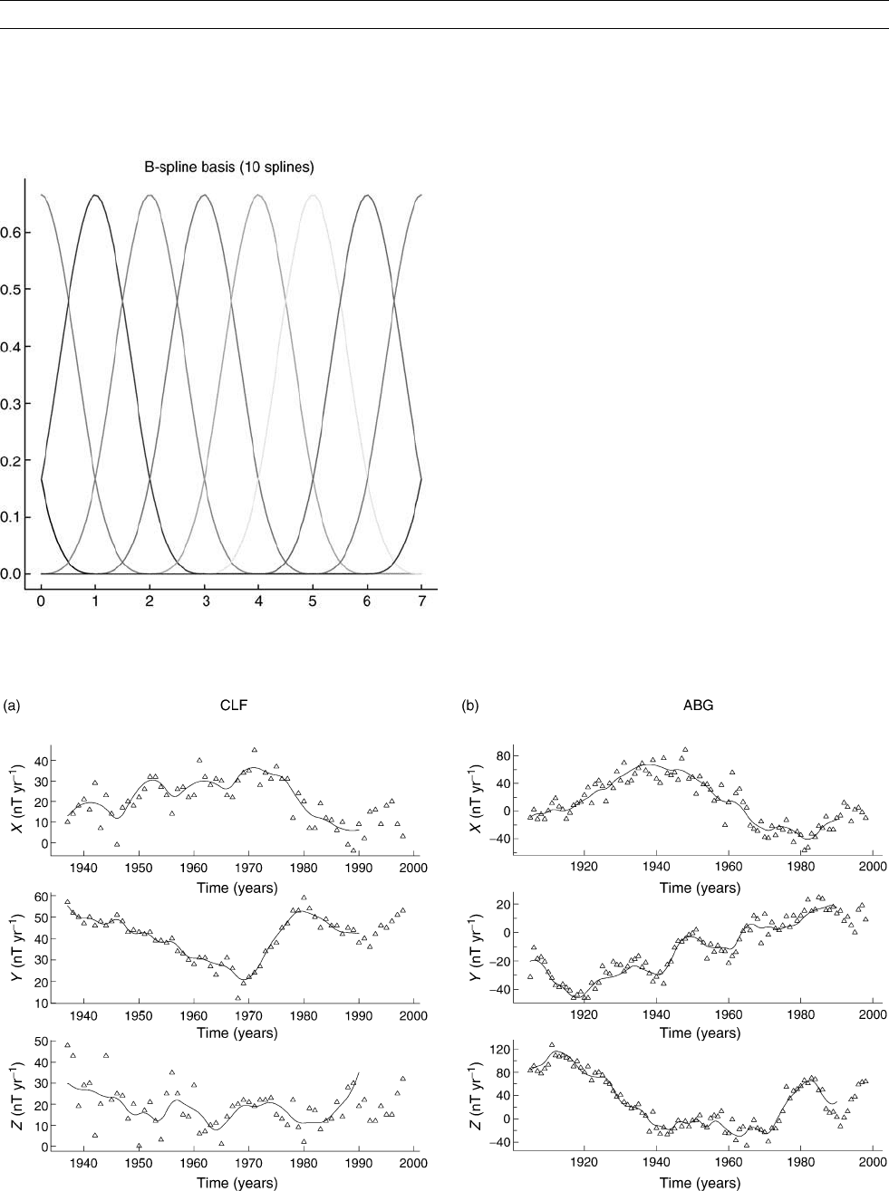
for its storage, whereas a B-spline basis is a local basis, meaning that

the basis functions are zero outside a small range (see Figure T4). This

fact leads to a design matrix which is sparse (in fact it is banded), and

its storage is minimized. Secondly, the B-splines provide a flexible

basis for smoothly varying descriptions of data. In fact one can show

that of all the interpolators passing through a time-series of points

(say f ðt

Þ; i ¼ 1; N), an expansion in cubic B-spline of order 4 (

f ðtÞ

say) is the unique interpolator which minimizes a particular measure

of roughness

]

f ðtÞ

dt: (Eq. 4)

Table T1 Characteristics of some models of the time-varying magnetic field. L is the maximum degree of the internal secular variation,

N is the number of temporal basis functions used for each Gauss coefficient

Model LN Time period Expansion Regularized? Author

GSFC(4/64) 5 2 1940–1963 Taylor No Cain et al. (1965)

GSFC(12/66) 1 3 1900–1966 Taylor No Cain et al. (1967)

GSFC(9/80) 1 4 1960–1980 Taylor No Langel et al. (1982)

MFSV/1900/1980/OBS 1 8 1900–1980 Legendre Yes Bloxham (1987)

1 10 1820–1900, Chebychev Yes Bloxham and Jackson (1989)

4 1900–1980

ufm1, ufm2 1 63 1690–1840, B-spline Yes Bloxham and Jackson (1992)

4 1840–1990

gufm1 1 16 1690–1990 B-spline Yes Jackson et al. (2000)

CM3 1 14 1960–1985 B-spline Yes Sabaka et al. (2002)

3 integrals

CM4 1 24 1960–2002.5 B-spline Yes Sabaka et al. (2004)

3 integrals

TIME-DEPENDENT MODELS OF THE GEOMAGNETIC FIELD 949

The idea of attempting to construct a smooth representation in time is

an application of “Occam ’s Razor,” that there should be no extra detail

in the representation than that truly demanded by the data. This idea of

“regularization” has been employed in the models of Table T1 from

that of Bloxham (1987) onward. All the models minimize a combina-

tion of norms on the core-mantle boundary (CMB) of the form:

ðn

]

ðn

dO dt ; (Eq. 5)

where B

is the radial field on the CMB. The models produced by

Bloxham, Jackson and coworkers use n

¼ 0 and n

¼ 2 in one norm,

and n

¼ 1 and n

¼ 0 (approximately) in a second norm; this is

slightly different to that of the comprehensive models (see below).

The ufm1/ufm2 and gufm1 field models share a common aim,

namely to model the long-term secular variation at the core surface

as accurately as possible. They were built using the B-spline basis with

knots every 2.5 years, and from the largest datasets possible at the

time: ufm1/ufm2 used over 250000 data originating from old ships’

logs, survey data, observatories and satellite missions; a description

of the oldest data can be found in Bloxham (1986) and Bloxham

et al. (1989). The gufm1 model was built from similar data from the

20th century, but a vastly expanded historical dataset, described in

Jonkers et al. (2003)—the model contains over 365000 data and

36512 parameters. No account is explicitly taken of external fields

in these models.

The comprehensive models

An effort began in the early 1990s to build a comprehensive series of

field models which took account of many effects which are recorded in

geomagnetic data in addition to the core secular variation. The first

model was reported by Sabaka and Baldwin (1993). We will specifi-

cally report on the latest model CM4 (Sabaka et al., 2004). In general

terms the model includes representations of the main field, its secular

variation, and both local-time (Sun-synchronous) and seasonal modes

of the magnetospheric and ionospheric fields, as well as describing

Figure T4 B-splines of order 4.

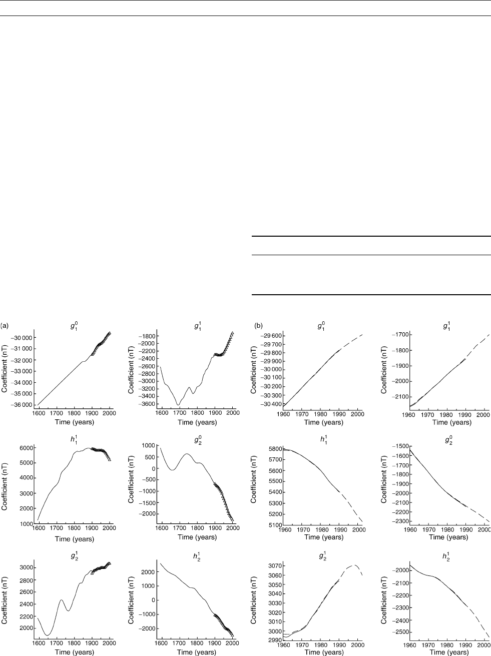
Figure T5 Comparison of secular variation models and annual means at (a) Chambon-la-Fore

t, France, (b) Alibag, India. Because

the post-1990 data were not used in the creation of gufm1, there is a small mismatch at the end of the data series—this shows the difficulty

in predicting the secular variation.

950 TIME-DEPENDENT MODELS OF THE GEOMAGNETIC FIELD

ring-current variations through the Dst index and internal fields induced

by time-varying external fields. The data used in creating the model con-

sists of POGO, Magsat, Ørsted, and CHAMP satellite data (totaling

over 1.6 million observations) and over 500000 observatory data; the

latter consist of either a 1.00 a.m. observation (actually an hourly mean)

on the quietest day of the month during the 1960–2002.5 period,

plusobservationsevery2honquietdaysduringthePOGOandMagsat

missions.

Figure T6 Comparison of one month (April 1990) of hourly mean data (X, Y, and Z components) from selected observatories and

predictions from CM4. (a) Charters Towers, (b) Kakioka, (c) Scott Base, (d) The D st index for April. Note the commencement of a

magnetic storm on the tenth day. The Dst index is used in the synthesis of predictions at individual observatories.

TIME-DEPENDENT MODELS OF THE GEOMAGNETIC FIELD 951

The comprehensive model takes into account not only the time-

varying core magnetic field (out to degree 13) but also the static

crustal field from degree 14 to degree 65. Because a model of the litho-

spheric field to this degree captures only a small proportion of the total

lithospheric signal, it is necessary to also solve for 1635 observatory

biases, generally three components at each observatory. The novel fea-

tures of the model arise in its very sophisticated treatment of the external

magnetic fields, and we will discuss these in some detail.

The ionospheric field is modeled as currents flowing in a thin shell

at an altitude of 110 km. This leads to magnetic fields which are

derived from potentials below and above this layer, which influence

the observatory and satellite data, respectively (since all the satellites

fly above this layer). In quasidipole coordinates, the currents are

allowed to vary with 24, 12, 8, and 6 h periods, as well as annually

and semiannually. Induced fields are accounted for by assuming that

the conductivity distribution of the Earth varies only in radius, which

means that an external spherical harmonic can only excite its corre-

sponding internal spherical harmonic. The magnetospheric field is also

parameterized in a similar way, with both daily and seasonal periodici-

ties, but also a modulation is allowed based on the Dst index.

In order to take into account the poloidal F-region currents through

which the satellites fly, a parametrization is made in terms of a toroidal

magnetic field, which also has periodic time variations.

The model is estimated by an iteratively reweighted least-squares

method, using Huber weights, and the core contribution is regularized

as in (5) using n

¼ 2 and n

¼ 1 in one norm and n

¼ 0 and n

¼ 2

in another. This difference from the ufm1/gufm1 method simply

represents a different approach; the fundamental quantity in the com-

prehensive models is the secular variation ]

, which has an expan-

sion in B-splines, and the main field B

is found as the integral of

this using the 1980 value as the offset or integration constant. All

the other parameters are regularized in a similar way, by smoothing

on spheres at different altitudes, representing the physical locations

of the sources. In total CM4 consists of 25243 free parameters.

Discussion

To illustrate the fidelity with which the various field models are able to

model observatory data, we show in Figure T5 a comparison of model

gufm1’s predictions with some observatory annual mean datasets. To

show CM4’s performance on very short timescales, Figure T6 com-

pares the model to hourly mean values for the month of April 1990,

Table T2 Comparison of r.m.s differences between observatory

annual means and predictions from the models gufm1 and CM3,

the latter with or without its external contributions

Component No. of data gufm1 CM3 (all) CM3 (no external)

X 4047 17.71 17.48 18.09

Y 4047 21.27 21.45 21.47

Z 4047 24.55 24.49 24.53

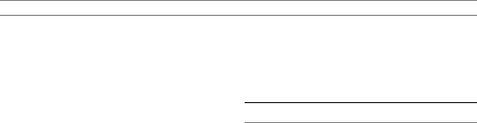
Figure T7 Comparison of model values for first six Gauss coefficients. (a) 1590–1990, (b) 1960–2002.5. Solid is gufm1, dashed is

CM4 and the triangles are DGRFs. In (a) g

has been fixed to decrease at a rate of 15nT yr

1

prior to 1840; in the absence of intensity data

it is necessary to fix the amplitude of the solutions.

952 TIME-DEPENDENT MODELS OF THE GEOMAGNETIC FIELD

data that were not used in deriving the model. It is clear that the model

is capable of predicting variations rather well, though with more diffi-

culty at the Antarctic station SBA (Scott Base). Table T2 compares the

performance of models gufm1 and CM3 against observatory data,

showing almost identical performance. This comes about principally

because of the large intrinsic variance of the data at some observa-

tories, which neither field model is able to capture. Figure T7 shows

a comparison of the model predictions for the variation in the first

six Gauss coefficients over century and decade timescales. Although

small differences exist, particularly in estimates of the instantaneous

secular variation, it is apparent that modeling has reached a stage

where there is considerable consensus between the models.

Andrew Jackson

Bibliography

Barraclough, D.R., 1978. Spherical harmonic analysis of the geomag-

netic field. Geomagnetic Bulletin Institute of Geological Science, 8.

Bloxham, J., 1986. Models of the magnetic field at the core-mantle

boundary for 1715, 1777 and 1842. Journal of Geophysical Research,

91: 13954–13966.

Bloxham, J., 1987. Simultaneous stochastic inversion for geomagnetic

main field and secular variation 1. A large-scale inverse problem.

Journal of Geophysical Research, 92: 11597–11608.

Bloxham, J., and Jackson, A., 1989. Simultaneous stochastic inversion

for geomagnetic main field and secular variation 2: 1820–1980.

Journal of Geophysical Research, 94: 15753–15769.

Bloxham, J., and Jackson, A., 1992. Time-dependent mapping of the

magnetic field at the core-mantle boundary. Journal of Geophysical

Research, 97: 19537–19563.

Bloxham, J., Gubbins, D., and Jackson, A., 1989. Geomagnetic secu-

lar variation. Philosophical Transactions of the Royal Society of

London, 329: 415–502.

Cain, J.C., Daniels, W.E., Hendricks, S.J., and Jensen, D.C., 1965. An

evaluation of the main geomagnetic field, 1940–1962. Journal of

Geophysical Research, 70: 3647–3674.

Cain, J.C., Hendricks, S.J., Langel, R.A., and Hudson, W.V., 1967. A

proposed model for the International Geomagnetic Reference Field—

1965. Journal of Geomagnetism and Geoelectricity, 19:335–355.

Jackson, A., Jonkers, A., and Walker, M., 2000. Four centuries of geo-

magnetic secular variation from historical records. Philosophical

Transactions of the Royal Society of London, 358: 957–990.

doi:10.1098/rsta.2000.0569

Jonkers, A.R.T., Jackson, A., and Murray, A., 2003. Four centuries of

geomagnetic data from historical records. Reviews of Geophysics,

41: 1006. doi:10.1029/2002RG000115. 2002 6.0

Langel, R.A., 1987. The main field. In Jacobs, J.A. (ed.) Geomagnet-

ism, Volume 1. London: Academic Press, pp. 249–512.

Langel, R.A., Estes, R.H., and Mead, G.D., 1982. Some new methods

in geomagnetic field modelling applied to the 1960–1980 epoch.

Journal of Geomagnetism and Geoelectricity, 34: 327–

349.

Langel, R.A., Kerridge, D.J., Barraclough, D.R., and Malin, S.R.C.,

1986. Geomagnetic temporal change: 1903–1982, a spline represen-

tation. Journal of Geomagnetism and Geoelectricity, 38:573–597.

Sabaka, T.J., and Baldwin, R.T., 1993. Modeling the Sq magnetic field

from POGO and Magsat satellite and contemporaneous hourly

observatory data, HSTX/G&G-9302, Hughes STX Corp., 7701

Greenbelt Road, Greenbelt, MD.

Sabaka, T.J., Olsen, N., and Langel, R.A., 2002. A comprehensive

model of the quiet-time, near-Earth magnetic field: phase 3, Geo-

physical Journal International, 151:32–68.

Sabaka, T.J., Olsen, N., and Purucker, M.E., 2004. Extending compre-

hensive models of the Earth’s magnetic field with Oersted and

CHAMP data, Geophysical Journal International, 159(2): 521–547.

doi:10.1111/j.1365-246X.2004.02421.x

Cross-references

IGRF, International Geomagnetic Reference Field

Main Field Modeling

Harmonics, Spherical

TRANSFER FUNCTIONS

Introduction

Transfer functions are used in magnetotellurics and geomagnetic depth

sounding to determine subsurface electrical conductivity from surface

measurements of natural electric and magnetic fields (Simpson and

Bahr, 2005). A transfer function describes the mathematical relation-

ship between surface measurements of variations of electric and mag-

netic fields.

Magnetotelluric transfer functions

Magnetotellurics uses natural electromagnetic field variations to image

subsurface electrical resistivity structure through electromagnetic

induction. The surface electric and magnetic fields at each frequency

are related through

;

where Z is defined as the magnetotelluric impedance, a transfer func-

tion. The components E

and E

are orthogonal components of the elec-

tric field and H

and H

are orthogonal components of the magnetic

field. These electromagnetic fields are nonstationary and the transfer

functions are computed as the average of many measurements. Robust

statistical methods are used to reliably estimate the transfer functions

(Jones et al., 1989; Larsen et al., 1996; Egbert, 1997) and remote-

reference processing should always be used (Gamble et al., 1979).

Magneto-variational studies

The vertical and horizontal magnetic fields are related through a

magnetic field transfer function T defined as

½H

¼½



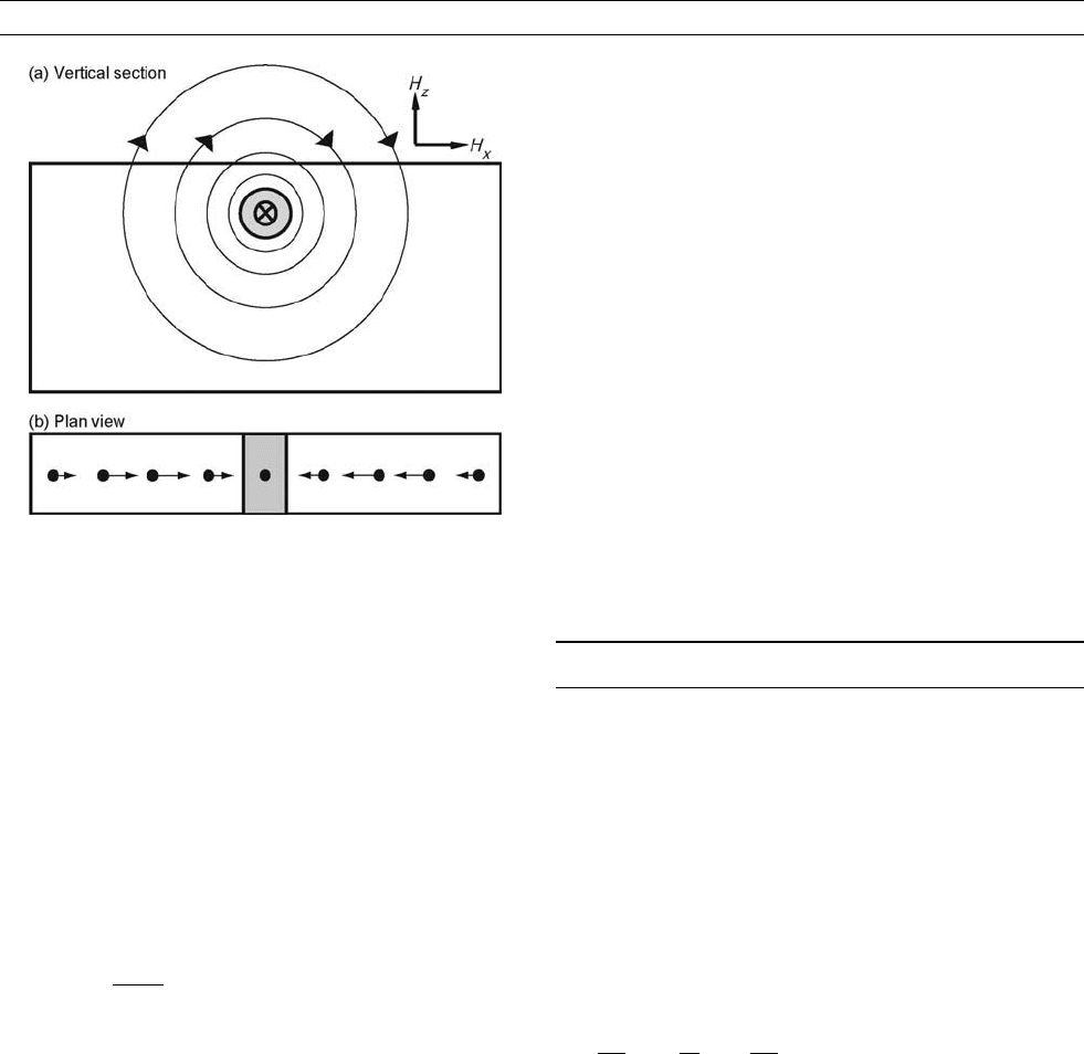
In the simple 2D geometry shown in Figure T8, the electric currents

flow along a conductivity anomaly and generate vertical magnetic

fields that are oriented upward on one side and downward on the other.

The magnetic field transfer function is often called the tipper. The

transfer function T can also be displayed as induction arrows which

are horizontal vectors with north and east components T

and T

respectively. Each component of the induction arrow is a complex

number with a real (in-phase) and imaginary (out-of-phase) part. In

the convention of Parkinson (1962), the real induction arrows point

toward a conductor (see Dudley Parkinson ) as shown in Figure T8.

In the Wiese convention the arrows point away from conductors

(Wiese, 1962). The direction of the induction arrows is further dis-

cussed by Lilley and Arora (1982). Induction arrows exhibit a reversal

above a conductivity anomaly as illustrated in Figure T8. The ocean is

the largest conductor on the surface of the Earth. Thus in surveys in

coastal areas, the real Parkinson arrows will point at the ocean and

the seawater must be included in conductivity models (see Coast effect

of induced currents). Edward Bullard is alleged to have commented

that “geomagnetic induction was a good way to find coastlines, but

there are easier ones.” Large-scale magneto-variational studies generate

TRANSFER FUNCTIONS 953

maps of induction arrows over a wide range of frequencies and have

been used to map the structure of the lithosphere on a number of conti-

nents (Gough, 1989).

Interstation transfer functions

If magnetotelluric data are recorded simultaneously at an array of sta-

tions, then interstation transfer functions can be defined. If a magnetic

field H

ðoÞ, is measured at one station and H

ðoÞ, is measured at

another station, then the interstation transfer function can be written as

ðoÞ¼

ðoÞ

at a frequency o. All stations in an array are related to the same base

station. One of the first applications of this method was described by

Schmucker (1970) in a study of the southwestern United States. Inter-

station magnetic field transfer functions can be inverted in a similar

way to apparent resistivity and phase to produce a resistivity model

of the Earth.

Martyn Unsworth

Bibliography

Egbert, G.D., 1997. Robust multiple-station magnetotelluric data pro-

cessing. Geophysical Journal International, 130: 475–496.

Gamble, T.B., Goubau, W.M., and Clarke, J., 1979. Magnetotellurics

with a remote reference. Geophysics, 44:53–68.

Gough, D.I., 1989. Magnetometer array studies, earth structure and

tectonic processes. Reviews of Geophysics, 27: 141–157.

Jones, A.G., Chave, A.D., Egbert, G.D., Auld, D., and Bahr, K., 1989.

A comparison of techniques for magnetotelluric response function

estimates. Journal of Geophysical Research, 94: 14201–14213.

Larsen, J.C., Mackie, R.L., Manzella, A., Fiordelisi, A., and Rieven, S.,

1996. Robust smooth magnetotelluric transfer functions. Geophysi-

cal Journal International, 124: 801–819.

Lilley, F.E.M., and Arora, B.R., 1982. The sign convention for quad-

rature Parkinson arrows in geomagnetic induction studies. Reviews

of Geophysics and Space Physics, 20: 513–518.

Parkinson, W.D., 1962. The influence of continents and oceans on

geomagnetic variations. Geophysical Journal of the Royal Astro-

nomical Society, 6: 441.

Schmucker, U., 1970. Anomalies of Geomagnetic Variations in the South-

western United States. Berkeley: University of California Press.

Simpson, F., and Bahr, K., 2005. Practical Magnetotellurics.

Cambridge: Cambridge University Press, p. 270.

Wiese, H., 1962. Geomagnetische Tiefentellurik Teil II: Die

Streichrichtung der Untergrundstrukturen des elektrischen Wide-

rstandes, erschlossen aus geomagnetischen Variationen [Strike

direction of underground structures of electric resistivity, inferred

from geomagnetic variations.]. Pure and applied geophysics, 52:

83–103.

Cross-references

Coast Effect of Induced Currents

Geomagnetic Deep Sounding

Induction Arrows

Magnetotellurics

Parkinson, Wilfred Dudley (1919–2001)

TRANSIENT EM INDUCTION

Geophysicists measure the electrical conductivity of subsurface materials

for a variety of purposes including geological mapping, mining investiga-

tion, groundwater resource evaluation and environmental assessment

(Meju, 2002). One of the methods used for mapping subsurface conduc-

tivity distributions is the transient electromagnetic (TEM) method that

employs artificially controlled sourcefields. The TEM method is sensitive

to electrical conductivity averaged over the volume of ground in which

induced electric currents are caused to flow.

Transient electromagnetic induction

The TEM method is founded on Maxwell’s equations that govern elec-

tromagnetic phenomena. Combining Ohm, Ampere, and Faraday laws

(Wangsness, 1986; Jackson, 1998) results in the damped wave equation

]

 m

]

¼ m

rJ

; (Eq. 1)

where B is magnetic field, m

is magnetic permeability, s is electrical

conductivity, e is dielectric permittivity, J

is the source current dis-

tribution, and t is time. For most geophysical applications of TEM,

the earth is generally considered to be nonmagnetic, such that m

¼ 4p

10

7

1

, the magnetic permeability of free space. The third term

on the left-hand side of (1) is the energy storage term describing wave

propagation. The second term on the left-hand side of (1) is the energy

dissipation term describing electromagnetic diffusion. In the TEM

method, @

B/@t

is relatively insignificant compared to @B/@t, so that

the wave propagation term is safely ignored. TEM induction is thus

a diffusive phenomenon.

A physical understanding of this phenomenon can be obtained by

recognizing that the induction process is equivalent to the diffusion

of an image of the transmitter (TX) loop into a conducting medium.

The similarity of the equations governing electromagnetic induction

and hydrodynamic vortex motion, first noticed by Helmholtz, leads

directly to the association of the image current with a smoke ring

(Lamb, 1945, p. 210). The latter is not “blown,” as commonly thought,

but instead moves by self-induction with a velocity that is generated

by the smoke ring’s own vorticity and described by the familiar

Figure T8 The geometry of the vertical magnetic fields associated

with naturally induced electric currents flowing in a buried

conductor. In the Parkinson convention the real induction arrows

point at the conductor, become stronger as the conductor is

approached, and then reverse direction above the conductor.

954 TRANSIENT EM INDUCTION

Biot-Savart law (Arms and Hama, 1965). An electromagnetic smoke

ring dissipates in a conducting medium much as the strength of a

hydrodynamic eddy is attenuated by the viscosity of its host fluid

(Taylor, 1958, pp. 96– 101). The medium property that dissipates the

electromagnetic smoke ring is electrical conductivit y.

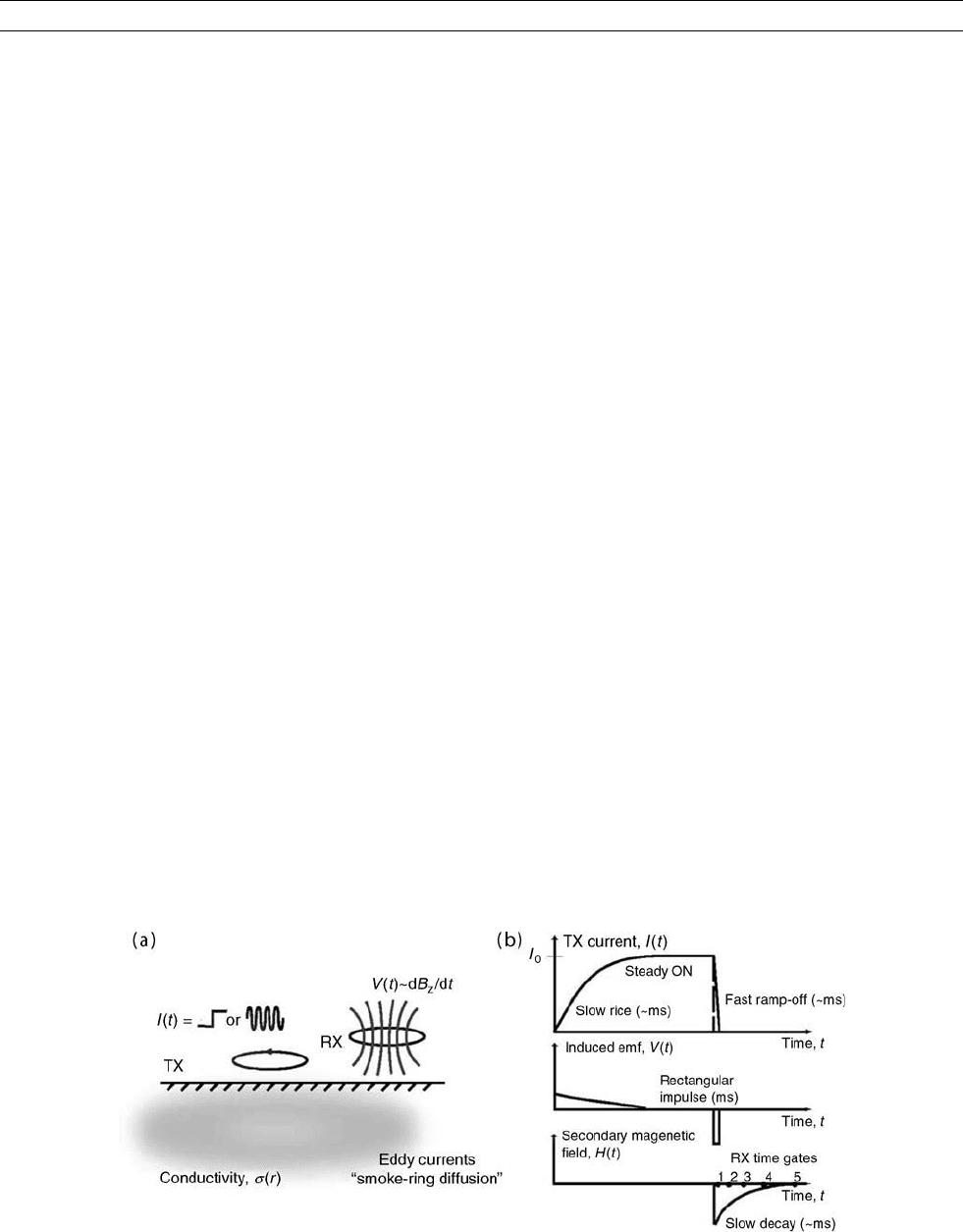
An inductively coupled TEM system is shown in Figure T9a.A

typical TX current waveform I (t) is a slow rise to a steady-on value

followed by a rapid shut-off, as exemplified by the linear ramp in

Figure T9b (top plot). Passing a disturbance through the TX loop

generates a primary magnetic field that is in-phase with, or propor-

tional to, the TX current. According to Faraday’s law of induction,

an electromotive force (emf) that scales with the time rate of change

of the primary magnetic field is also generated. The emf drives electro-

magnetic eddy currents in the conductive earth, notably in this case

during the ramp-off interval, as shown in Figure T9b (middle plot).

After the ramp is terminated, the emf vanishes and the eddy currents

start to decay via Ohmic dissipation of heat. A weak, secondary mag-

netic field is produced in proportion to the waning strength of the eddy

currents. The receiver (RX) coil voltage measures the time rate of

change of the decaying secondary magnetic field as depicted in

Figure T9b (bottom plot). In typical TEM systems, the RX voltage

measurements are made during the TX off-time when the primary field

is absent. The advantage of measuring during TX off-time is that the

relatively weak secondary signal is not swamped by the much stronger

primary signal.

During the ramp-off, the induced current assumes the shape of the

horizontal projection of the TX loop onto the surface of the conducting

ground. The sense of the circulating induced currents is such that

the secondary magnetic field they create tends to maintain the total

magnetic field at its original steady-on value prior to the TX ramp-

off. Thus, the induced currents flow in the same direction as the TX

current, i.e., opposing the TX current decrease that served as the emf

source. The image current then diffuses downward and outward while

diminishing in amplitude. A mathematical treatment of the electromag-

netic smoke ring phenomenon appears in Nabighian (1979).

Transient electromagnetic forward modeling

Calculation of the TEM field generated by a magnetic or electric

dipole source situated on, above or within a layered conducting med-

ium is a well-known boundary value problem of classical physics.

One standard solution technique is to calculate the mutual impe-

dance, Z between the transmitter and receiver loops as a function of

measurement (or delay) times t. For a TX loop of radius a and RX

loop of radius b that are co-axial and located on the ground’s surface,

we have that (Knight and Raiche, 1982)

ZðtÞ¼pm

1

fIð pÞpA

ðm; p; lÞgJ

ðlaÞJ

ðlbÞdl:

In the above equation, A

(m,p,l) is the layered-earth impedance function,

m represents the parameters of the hypothetical earth-model (namely

electrical conductivities, s

and thicknesses, h

of the layers), p is the

Laplace transform variable corresponding to –io where o is the angular

frequency, “i” is the imaginary unit, l is the integration variable for the

inverse Hankel transform, I( p) represents the Laplace transform of the

normalized current waveform and is equal to –p

–1

for step function

turn-off of TX current, J

is the Bessel function of order 1, and L

1

the inverse Laplace transform operator with respect to p.

Similar analytic solutions are available for other TX-RX configurations

and a variety of special-purpose algorithms are available for evaluating such

Hankel transforms or integrals over Bessel functions. Note that the manner

in which the TX current is switched off influences the TEM response and

needs to be accounted for in the forward models (Raiche, 1984).

The TEM response of 3D subsurface conductivity distributions

requires the application of numerical methods for solving the govern-

ing Maxwell partial differential equations (see Hohmann, 1987). Full

3D numerical simulations involve a complete description of the phy-

sics of electromagnetic induction including galvanic and vortex contri-

butions. The galvanic term appears when induced currents encounter

spatial gradients in electrical conductivity. Electric charges accumulate

across interfaces in electrical conductivity. In 1D layered media

excited by a purely inductive electromagnetic source such as a loop,

induced currents flow horizontally and do not cross layer boundaries.

In that case, only the vortex contribution is present.

Transient electromagnetic method of geophysical

prospecting

In TEM surveying, a primary field is generated by a rectangular or

square TX loop, with dimensions of ten to a few hundred meters

(Figure T10). A long straight wire grounded at both ends can also

serve as the transmitter. For shallow depth probes, a 20 m-sided TX

loop could suffice for imaging about 60–100 m depth depending

on ground conditions (Meju et al., 2000). The primary field is not

continuous but consists of a series of pulses between which the

Figure T9 (a) TX loop lying on the surface of an isotropic uniform half-space of electrical conductivity, s. A disturbance I(t)inthe

source current immediately generates an electromagnetic eddy cur rent in the ground just beneath the TX loop. An RX coil measures

the induced voltage V(t), which is a measure of the time-derivative of the magnetic flux generated by the diffusing eddy current.

(b) Typical TX current waveform I(t) with slow rise time and fast ramp-off; induced emf V( t), proportional to the time rate of change

of the primary magnetic field; decay ing secondary magnetic field H(t) due to the dissipation of currents induced in the ground

(Everett and Meju, 2005).

TRANSIENT EM INDUCTION 955