Greene W.H. Econometric Analysis

Подождите немного. Документ загружается.

APPENDIX D

✦

Large-Sample Distribution Theory

1069

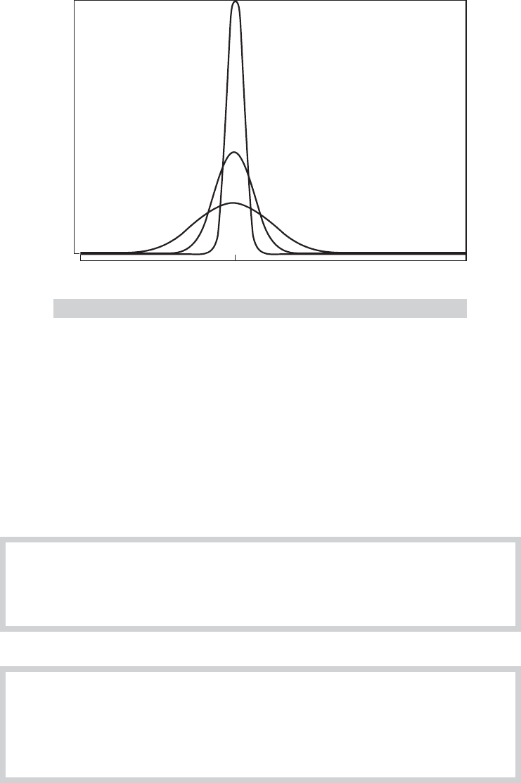
n  10

n  100

Estimator

Density

n  1000

␪

FIGURE D.1

Quadratic Convergence to a Constant,

Convergence in probability does not imply convergence in mean square. Consider the simple

example given earlier in which x

equals either zero or n with probabilities 1 − (1/n) and (1/n).

The exact expected value of x

is 1 for all n, which is not the probability limit. Indeed, if we let

Prob(x

= n

) = (1/n) instead, the mean of the distribution explodes, but the probability limit is

still zero. Again, the point x

= n

becomes ever more extreme but, at the same time, becomes

ever less likely.

The conditions for convergence in mean square are usually easier to verify than those for

the more general form. Fortunately, we shall rarely encounter circumstances in which it will be

necessary to show convergence in probability in which we cannot rely upon convergence in mean

square. Our most frequent use of this concept will be in formulating consistent estimators.

DEFINITION D.2

Consistent Estimator

An estimator

of a parameter θ is a consistent estimator of θ if and only if

plim

= θ. (D-4)

THEOREM D.4

Consistency of the Sample Mean

The mean of a random sample from any population with ﬁnite mean μ and ﬁnite variance

is a consistent estimator of μ.

Proof: E[¯x

] = μ and Var[ ¯x

] = σ

/n. Therefore, ¯x

converges in mean square to μ,or

plim ¯x

= μ.

1070

PART VI

✦

Appendices

Theorem D.4 is broader than it might appear at ﬁrst.

COROLLARY TO THEOREM D.4

Consistency of a Mean

of Functions

In random sampling, for any function g(x),ifE[g(x)] and Var[g(x)] are ﬁnite constants,

then

plim



i=1

g(x

) = E[g(x)]. (D-5)

Proof: Deﬁne y

= g(x

) and use Theorem D.4.

Example D.2 Estimating a Function of the Mean

In sampling from a normal distribution with mean μ and variance 1, E [e

] = e

μ+1/2

and

Var [e

] = e

2μ+2

− e

2μ+1

. (See Section B.4.4 on the lognormal distribution.) Hence,

plim



i =1

= e

μ+1/2

D.2.2 OTHER FORMS OF CONVERGENCE AND LAWS

OF LARGE NUMBERS

Theorem D.4 and the corollary just given are particularly narrow forms of a set of results known

as laws of large numbers that are fundamental to the theory of parameter estimation. Laws of

large numbers come in two forms depending on the type of convergence considered. The simpler

of these are “weak laws of large numbers” which rely on convergence in probability as we deﬁned

it above. “Strong laws” rely on a broader type of convergence called almost sure convergence.

Overall, the law of large numbers is a statement about the behavior of an average of a large

number of random variables.

THEOREM D.5

Khinchine’s Weak Law of Large Numbers

If x

, i = 1,...,n is a random (i.i.d.) sample from a distribution with ﬁnite mean E [x

] = μ,

then

plim ¯x

= μ.

Proofs of this and the theorem below are fairly intricate. Rao (1973) provides one.

Notice that this is already broader than Theorem D.4, as it does not require that the variance of

the distribution be ﬁnite. On the other hand, it is not broad enough, because most of the situations

we encounter where we will need a result such as this will not involve i.i.d. random sampling. A

broader result is

APPENDIX D

✦

Large-Sample Distribution Theory

1071

THEOREM D.6

Chebychev’s Weak Law of Large Numbers

If x

, i = 1,...,n is a sample of observations such that E [x

] = μ

< ∞ and Var[x

] =

< ∞ such that ¯σ

/n = (1/n

)

→ 0 as n →∞, then plim( ¯x

− ¯μ

) = 0.

There is a subtle distinction between these two theorems that you should notice. The Chebychev

theorem does not state that ¯x

converges to ¯μ

, or even that it converges to a constant at all.

That would require a precise statement about the behavior of ¯μ

. The theorem states that as

n increases without bound, these two quantities will be arbitrarily close to each other—that

is, the difference between them converges to a constant, zero. This is an important notion

that enters the derivation when we consider statistics that converge to random variables, in-

stead of to constants. What we do have with these two theorems are extremely broad condi-

tions under which a sample mean will converge in probability to its population counterpart.

The more important difference between the Khinchine and Chebychev theorems is that the

second allows for heterogeneity in the distributions of the random variables that enter

the mean.

In analyzing time-series data, the sequence of outcomes is itself viewed as a random event.

Consider, then, the sample mean, ¯x

. The preceding results concern the behavior of this statistic

as n →∞for a particular realization of the sequence ¯x

,..., ¯x

. But, if the sequence, itself, is

viewed as a random event, then limit to which ¯x

converges may be also. The stronger notion of

almost sure convergence relates to this possibility.

DEFINITION D.3

Almost Sure Convergence

The random variable x

converges almost surely to the constant c if and only if

Prob



lim

n→∞

= c



= 1.

This is denoted x

a.s.

−→ c. It states that the probability of observing a sequence that does not

converge to c ultimately vanishes. Intuitively, it states that once the sequence x

becomes close

to c, it stays close to c.

Almost sure convergence is used in a stronger form of the law of large numbers:

THEOREM D.7

Kolmogorov’s Strong Law of Large Numbers

If x

, i = 1,...,n is a sequence of independently distributed random variables such that

E [x

] = μ

< ∞ and Var[x

] = σ

< ∞ such that



∞

i=1

< ∞ as n →∞then

¯x

− ¯μ

a.s.

−→ 0.

1072

PART VI

✦

Appendices

THEOREM D.8

Markov’s Strong Law of Large Numbers

If {z

}is a sequence of independent random variables with E[z

] = μ

< ∞and if for some

δ>0,



∞

i=1

E[|z

− μ

1+δ

]/i

1+δ

< ∞, then ¯z

− ¯μ

converges almost surely to 0, which

we denote ¯z

− ¯μ

a.s.

−→ 0.

The variance condition is satisﬁed if every variance in the sequence is ﬁnite, but this is not strictly

required; it only requires that the variances in the sequence increase at a slow enough rate that

the sequence of variances as deﬁned is bounded. The theorem allows for heterogeneity in the

means and variances. If we return to the conditions of the Khinchine theorem, i.i.d. sampling, we

have a corollary:

COROLLARY TO THEOREM D.8

(Kolmogorov)

If x

, i = 1,...,n is a sequence of independent and identically distributed random variables

such that E[x

] = μ<∞ and E[|x

|] < ∞, then ¯x

− μ

a.s.

−→ 0.

Note that the corollary requires identically distributed observations while the theorem only

requires independence. Finally, another form of convergence encountered in the analysis of time-

series data is convergence in rth mean:

DEFINITION D.4

Convergence in rth Mean

If x

is a sequence of random variables such that E[|x

] < ∞and lim

n→∞

E[|x

−c|

] = 0,

then x

converges in rth mean to c. This is denoted x

r.m.

−→ c.

Surely the most common application is the one we met earlier, convergence in means square,

which is convergence in the second mean. Some useful results follow from this deﬁnition:

THEOREM D.9

Convergence in Lower Powers

If x

converges in rth mean to c, then x

converges in sth mean to c for any s < r . The

proof uses Jensen’s Inequality, Theorem D.13. Write E[|x

− c|

] = E[(|x

− c|

)

s/r

] ≤



E[(|x

− c|

)]



s/r

and the inner term converges to zero so the full function must also.

The use of the expected absolute deviation differs a bit from the expected squared deviation that we have

used heretofore to characterize the spread of a distribution. Consider two examples. If z ∼ N[0,σ

], then

E[|z|] = Prob[z < 0]E[−z | z < 0] + Prob[z ≥ 0]E[z |z ≥ 0] = 0.7979σ . (See Theorem 18.2.) So, ﬁnite

expected absolute value is the same as ﬁnite second moment for the normal distribution. But if z takes values

[0, n] with probabilities [1 − 1/n, 1/n], then the variance of z is (n − 1), but E[|z − μ

|]is2− 2/n.For

this case, ﬁnite expected absolute value occurs without ﬁnite expected second moment. These are different

characterizations of the spread of the distribution.

APPENDIX D

✦

Large-Sample Distribution Theory

1073

THEOREM D.10

Generalized Chebychev’s Inequality

If x

is a random variable and c is a constant such that with E[|x

− c|

] < ∞ and ε is a

positive constant, then Prob(|x

− c| >ε)≤ E[|x

− c|

]/ε

We have considered two cases of this result already, when r = 1 which is the Markov inequality,

Theorem D.3, and when r = 2, which is the Chebychev inequality we looked at ﬁrst in Theo-

rem D.2.

THEOREM D.11

Convergence in rth mean and Convergence

in Probability

If x

r.m.

−→ c, for some r > 0, then x

−→ c. The proof relies on Theorem D.10. By

assumption, lim

n→∞

E [|x

−c|

] = 0 so for some n sufﬁciently large, E [|x

−c|

] < ∞.

By Theorem D.10, then, Prob(|x

−c|>ε)≤ E [|x

−c|

]/ε

for any ε>0. The denomina-

tor of the fraction is a ﬁxed constant and the numerator converges to zero by our initial

assumption, so lim

n→∞

Prob(|x

−c|>ε)=0, which completes the proof.

One implication of Theorem D.11 is that although convergence in mean square is a convenient

way to prove convergence in probability, it is actually stronger than necessary, as we get the same

result for any positive r.

Finally, we note that we have now shown that both almost sure convergence and convergence

in r th mean are stronger than convergence in probability; each implies the latter. But they,

themselves, are different notions of convergence, and neither implies the other.

DEFINITION D.5

Convergence of a Random Vector or Matrix

Let x

denote a random vector and X

a random matrix, and c and C denote a vector

and matrix of constants with the same dimensions as x

and X

, respectively. All of the

preceding notions of convergence can be extended to (x

, c) and (X

, C) by applying the

results to the respective corresponding elements.

D.2.3 CONVERGENCE OF FUNCTIONS

A particularly convenient result is the following.

THEOREM D.12

Slutsky Theorem

For a continuous function g(x

) that is not a function of n,

plim g(x

) = g(plim x

). (D-6)

The generalization of Theorem D.12 to a function of several random variables is direct, as

illustrated in the next example.

1074

PART VI

✦

Appendices

Example D.3 Probability Limit of a Function of

xand

In random sampling from a population with mean μ and variance σ

, the exact expected

value of ¯x

will be difﬁcult, if not impossible, to derive. But, by the Slutsky theorem,

plim

¯x

An application that highlights the difference between expectation and probability is suggested

by the following useful relationships.

THEOREM D.13

Inequalities for Expectations

Jensen’s Inequality. If g(x

) is a concave function of x

, then g



E [x

]



≥ E [g(x

)].

Cauchy–Schwarz Inequality. For two random variables,

E [|xy|] ≤



E [x

]



1/2



E [y

]



1/2

Although the expected value of a function of x

may not equal the function of the expected

value—it exceeds it if the function is concave—the probability limit of the function is equal to

the function of the probability limit.

The Slutsky theorem highlights a comparison between the expectation of a random variable

and its probability limit. Theorem D.12 extends directly in two important directions. First, though

stated in terms of convergence in probability, the same set of results applies to convergence in

rth mean and almost sure convergence. Second, so long as the functions are continuous, the

Slutsky theorem can be extended to vector or matrix valued functions of random scalars, vectors,

or matrices. The following describe some speciﬁc applications. Some implications of the Slutsky

theorem are now summarized.

THEOREM D.14

Rules for Probability Limits

If x

and y

are random variables with plim x

= c and plim y

= d, then

plim(x

+ y

) = c + d,(sum rule) (D-7)

plim x

= cd,(product rule) (D-8)

plim x

= c/d if d = 0.(ratio rule) (D-9)

If W

is a matrix whose elements are random variables and if plim W

= , then

plim W

−1

= 

−1

.(matrix inverse rule) (D-10)

If X

and Y

are random matrices with plim X

= A and plim Y

= B, then

plim X

= AB.(matrix product rule) (D-11)

D.2.4 CONVERGENCE TO A RANDOM VARIABLE

The preceding has dealt with conditions under which a random variable converges to a constant,

for example, the way that a sample mean converges to the population mean. To develop a theory

APPENDIX D

✦

Large-Sample Distribution Theory

1075

for the behavior of estimators, as a prelude to the discussion of limiting distributions, we now

consider cases in which a random variable converges not to a constant, but to another random

variable. These results will actually subsume those in the preceding section, as a constant may

always be viewed as a degenerate random variable, that is one with zero variance.

DEFINITION D.6

Convergence in Probability to a Random

Variable

The random variable x

converges in probability to the random variable x if

lim

n→∞

Prob(|x

− x| >ε)= 0 for any positive ε.

As before, we write plim x

= x to denote this case. The interpretation (at least the intuition) of

this type of convergence is different when x is a random variable. The notion of closeness deﬁned

here relates not to the concentration of the mass of the probability mechanism generating x

at a

point c, but to the closeness of that probability mechanism to that of x. One can think of this as

a convergence of the CDF of x

to that of x.

DEFINITION D.7

Almost Sure Convergence to a Random Variable

The random variable x

converges almost surely to the random variable x if and only if

lim

n→∞

Prob(|x

− x| >εfor all i ≥ n) = 0 for all ε>0.

DEFINITION D.8

Convergence in rth Mean to a Random Variable

The random variable x

converges in rth mean to the random variable x if and only if

lim

n→∞

E [|x

− x|

] = 0. This is labeled x

r.m.

−→ x. As before, the case r = 2 is labeled

convergence in mean square.

Once again, we have to revise our understanding of convergence when convergence is to a random

variable.

THEOREM D.15

Convergence of Moments

Suppose x

r.m.

−→ x and E [|x|

] is ﬁnite. Then, lim

n→∞

E [|x

] = E [|x|

Theorem D.15 raises an interesting question. Suppose we let r grow, and suppose that x

r.m.

−→ x

and, in addition, all moments are ﬁnite. If this holds for any r, do we conclude that these random

variables have the same distribution? The answer to this longstanding problem in probability

theory—the problem of the sequence of moments—is no. The sequence of moments does not

uniquely determine the distribution. Although convergence in rth mean and almost surely still

both imply convergence in probability, it remains true, even with convergence to a random variable

instead of a constant, that these are different forms of convergence.

1076

PART VI

✦

Appendices

D.2.5 CONVERGENCE IN DISTRIBUTION:

LIMITING DISTRIBUTIONS

A second form of convergence is convergence in distribution. Let x

be a sequence of random

variables indexed by the sample size, and assume that x

has cdf F

DEFINITION D.9

Convergence in Distribution

converges in distribution to a random variable x with CDF F(x) if

lim

n→∞

| F

) − F(x)|=0 at all continuity points of F(x).

This statement is about the probability distribution associated with x

; it does not imply that

converges at all. To take a trivial example, suppose that the exact distribution of the random

variable x

Prob(x

= 1) =

n + 1

, Prob(x

= 2) =

−

n + 1

As n increases without bound, the two probabilities converge to

, but x

does not converge to a

constant.

DEFINITION D.10

Limiting Distribution

If x

converges in distribution to x, where F

) is the CDF of x

, then F(x) is the limiting

distribution of x

. This is written

−→ x.

The limiting distribution is often given in terms of the pdf, or simply the parametric family. For

example, “the limiting distribution of x

is standard normal.”

Convergence in distribution can be extended to random vectors and matrices, although not

in the element by element manner that we extended the earlier convergence forms. The reason is

that convergence in distribution is a property of the CDF of the random variable, not the variable

itself. Thus, we can obtain a convergence result analogous to that in Deﬁnition D.9 for vectors or

matrices by applying deﬁnition to the joint CDF for the elements of the vector or matrices. Thus,

−→ x if lim

n→∞

) − F(x)|=0 and likewise for a random matrix.

Example D.4 Limiting Distribution of t

−

Consider a sample of size n from a standard normal distribution. A familiar inference problem

is the test of the hypothesis that the population mean is zero. The test statistic usually used

is the t statistic:

n−1

¯x

√

where



i =1

( x

− ¯x

)

n − 1

APPENDIX D

✦

Large-Sample Distribution Theory

1077

The exact distribution of the random variable t

n−1

is t with n − 1 degrees of freedom. The

density is different for every n:

f ( t

n−1

) =

( n/2)

[( n − 1)/2]

[(n − 1) π]

−1/2



1 +

n−1

n − 1



−n/2

, (D-12)

as is the CDF, F

n−1

(t) =

−∞

n−1

( x) dx. This distribution has mean zero and variance (n −1)/

(n − 3) . As n grows to inﬁnity, t

n−1

converges to the standard normal, which is written

n−1

−→ N[0, 1].

DEFINITION D.11

Limiting Mean and Variance

The limiting mean and variance of a random variable are the mean and variance of the

limiting distribution, assuming that the limiting distribution and its moments exist.

For the random variable with t[n] distribution, the exact mean and variance are zero and

n/(n − 2), whereas the limiting mean and variance are zero and one. The example might suggest

that the limiting mean and variance are zero and one; that is, that the moments of the limiting

distribution are the ordinary limits of the moments of the ﬁnite sample distributions. This situation

is almost always true, but it need not be. It is possible to construct examples in which the exact

moments do not even exist, even though the moments of the limiting distribution are well deﬁned.

Even in such cases, we can usually derive the mean and variance of the limiting distribution.

Limiting distributions, like probability limits, can greatly simplify the analysis of a problem.

Some results that combine the two concepts are as follows.

THEOREM D.16

Rules for Limiting Distributions

1. If x

−→ x and plim y

= c, then

−→ cx, (D-13)

which means that the limiting distribution of x

is the distribution of cx. Also,

+ y

−→ x + c, (D-14)

−→ x/c, if c = 0. (D-15)

2. If x

−→ x and g(x

) is a continuous function, then

g(x

)

−→ g(x). (D-16)

This result is analogous to the Slutsky theorem for probability limits. For

an example, consider the t

random variable discussed earlier. The exact distribu-

tion of t

is F[1, n]. But as n −→ ∞ , t

converges to a standard normal variable.

According to this result, the limiting distribution of t

will be that of the square of a

standard normal, which is chi-squared with one

See, for example, Maddala (1977a, p. 150).

For proofs and further discussion, see, for example, Greenberg and Webster (1983).

1078

PART VI

✦

Appendices

THEOREM D.16

(Continued)

degree of freedom. We conclude, therefore, that

F[1, n]

−→ chi-squared[1]. (D-17)

We encountered this result in our earlier discussion of limiting forms of the standard

normal family of distributions.

3. If y

has a limiting distribution and plim (x

− y

) = 0, then x

has the same limiting

distribution as y

The third result in Theorem D.16 combines convergence in distribution and in probability. The

second result can be extended to vectors and matrices.

Example D.5 The F Distribution

Suppose that t

1,n

and t

2,n

are a K × 1 and an M × 1 random vector of variables whose

components are independent with each distributed as t with n degrees of freedom. Then, as

we saw in the preceding, for any component in either random vector, the limiting distribution

is standard normal, so for the entire vector, t

j,n

−→ z

, a vector of independent standard

normally distributed variables. The results so far show that



1,n

)/K



2,n

)/M

−→ F [K, M].

Finally, a speciﬁc case of result 2 in Theorem D.16 produces a tool known as the Cram´er–Wold

device.

THEOREM D.17

Cramer–Wold Device

If x

−→ x, then c



−→ c



x for all conformable vectors c with real valued elements.

By allowing c to be a vector with just a one in a particular position and zeros elsewhere, we see

that convergence in distribution of a random vector x

to x does imply that each component does

likewise.

D.2.6 CENTRAL LIMIT THEOREMS

We are ultimately interested in ﬁnding a way to describe the statistical properties of estimators

when their exact distributions are unknown. The concepts of consistency and convergence in

probability are important. But the theory of limiting distributions given earlier is not yet adequate.

We rarely deal with estimators that are not consistent for something, though perhaps not always

the parameter we are trying to estimate. As such,

if plim

= θ, then

−→ θ.

That is, the limiting distribution of

is a spike. This is not very informative, nor is it at all what

we have in mind when we speak of the statistical properties of an estimator. (To endow our ﬁnite

sample estimator

with the zero sampling variance of the spike at θ would be optimistic in the

extreme.)

As an intermediate step, then, to a more reasonable description of the statistical properties

of an estimator, we use a stabilizing transformation of the random variable to one that does have