Greene W.H. Econometric Analysis

Подождите немного. Документ загружается.

APPENDIX C

✦

Estimation and Inference

1049

skewed while ﬁnancial data such as asset returns and exchange rate movements are relatively

more symmetrically distributed but are also more widely dispersed than other variables that might

be observed. Two measures used to quantify these effects are the

skewness =





i=1

− ¯x )

(

n − 1

)



, and kurtosis =





i=1

− ¯x )

(

n − 1

)



(Benchmark values for these two measures are zero for a symmetric distribution, and three for

one which is “normally” dispersed.) The skewness coefﬁcient has a bit less of the intuitive appeal

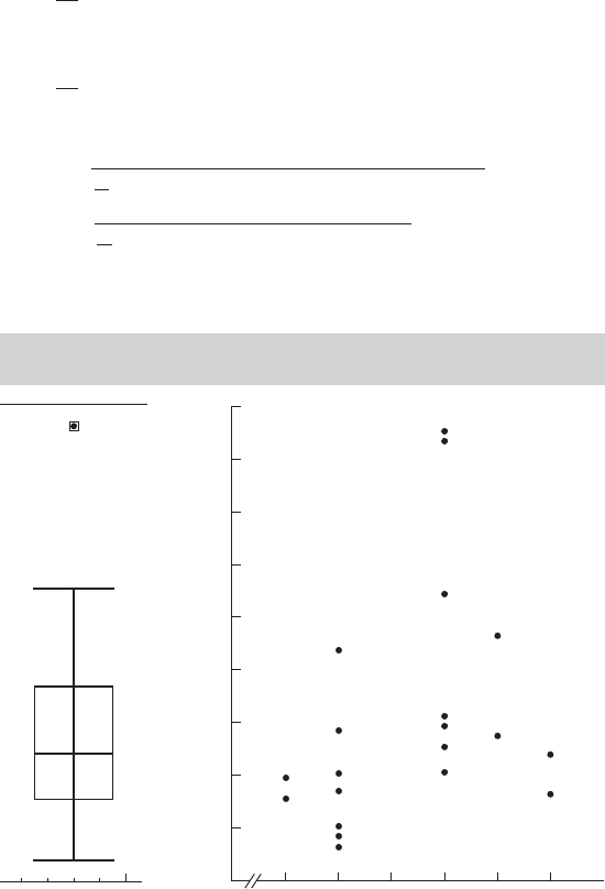
of the mean and standard deviation, and the kurtosis measure has very little at all. The box and

whisker plot is a graphical device which is often used to capture a large amount of information

about the sample in a simple visual display. This plot shows in a ﬁgure the median, the range of

values contained in the 25th and 75th percentile, some limits that show the normal range of values

expected, such as the median plus and minus two standard deviations, and in isolation values that

could be viewed as outliers. A box and whisker plot is shown in Figure C.1 for the income variable

in Example C.1.

If the sample contains data on more than one variable, we will also be interested in measures

of association among the variables. A scatter diagram is useful in a bivariate sample if the sample

contains a reasonable number of observations. Figure C.1 shows an example for a small data set.

If the sample is a multivariate one, then the degree of linear association among the variables can

be measured by the pairwise measures

covariance: s



i=1

− ¯x )(y

− ¯y)

n − 1

, (C-3)

correlation: r

If the sample contains data on several variables, then it is sometimes convenient to arrange the

covariances or correlations in a

covariance matrix: S = [s

], (C-4)

correlation matrix: R = [r

Some useful algebraic results for any two variables (x

, y

), i = 1,...,n, and constants a and

b are





i=1



− n ¯x

n − 1

, (C-5)





i=1



− n ¯x ¯y

n − 1

, (C-6)

−1 ≤ r

≤ 1,

ax,by

, a, b = 0, (C-7)

=|a|s

(C-8)

ax,by

= (ab)s

1050

PART VI

✦

Appendices

Note that these algebraic results parallel the theoretical results for bivariate probability distri-

butions. [We note in passing, while the formulas in (C-2) and (C-5) are algebraically the same,

(C-2) will generally be more accurate in practice, especially when the values in the sample are

very widely dispersed.]

Example C.1 Descriptive Statistics for a Random Sample

Appendix Table FC.1 contains a (hypothetical) sample of observations on income and educa-

tion (The observations all appear in the calculations of the means below.) A scatter diagram

appears in Figure C.1. It suggests a weak positive association between income and educa-

tion in these data. The box and whisker plot for income at the left of the scatter plot shows

the distribution of the income data as well.

Means:

I =

⎡

⎣

20.5 + 31.5 + 47.7 + 26.2 + 44.0 + 8.28 + 30.8 +

17.2 + 19.9 + 9.96 + 55.8 + 25.2 + 29.0 + 85.5 +

15.1 + 28.5 + 21.4 + 17.7 + 6.42 + 84.9

⎤

⎦

= 31.278,

E =



12 + 16 + 18 + 16 + 12 + 12 + 16 + 12 + 10 + 12 +

16 + 20 + 12 + 16 + 10 + 18 + 16 + 20 + 12 + 16



= 14.600.

Standard deviations:

[(20.5 − 31.278)

+···+(84.9 − 31.278)

] = 22.376,

[(12 − 14.6)

+···+(16− 14.6)

] = 3.119.

FIGURE C.1

Box and Whisker Plot for Income and Scatter

Diagram for Income and Education.

Income in thousands

2010 12 14 16 18

Education

APPENDIX C

✦

Estimation and Inference

1051

Covariance: s

[20.5(12) +···+84.9(16) − 20( 31.28)(14.6)] = 23.597,

Correlation: r

23.597

(22.376)( 3.119)

= 0.3382.

The positive correlation is consistent with our observation in the scatter diagram.

The statistics just described will provide the analyst with a more concise description of

the data than a raw tabulation. However, we have not, as yet, suggested that these measures

correspond to some underlying characteristic of the process that generated the data. We do

assume that there is an underlying mechanism, the data generating process, that produces the

data in hand. Thus, these serve to do more than describe the data; they characterize that process,

or population. Because we have assumed that there is an underlying probability distribution, it

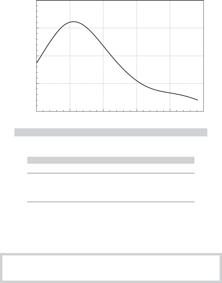
might be useful to produce a statistic that gives a broader view of the DGP. The histogram is a

simple graphical device that produces this result—see Examples C.3 and C.4 for applications. For

small samples or widely dispersed data, however, histograms tend to be rough and difﬁcult to

make informative. A burgeoning literature [see, e.g., Pagan and Ullah (1999) and Li and Racine

(2007)] has demonstrated the usefulness of the kernel density estimator as a substitute for the

histogram as a descriptive tool for the underlying distribution that produced a sample of data.

The underlying theory of the kernel density estimator is fairly complicated, but the computations

are surprisingly simple. The estimator is computed using

f (x

∗

) =



i=1



− x

∗



where x

,...,x

are the n observations in the sample,

f (x

∗

) denotes the estimated density func-

tion, x

∗

is the value at which we wish to evaluate the density, and h and K[·] are the “bandwidth”

and “kernel function” that we now consider. The density estimator is rather like a histogram,

in which the bandwidth is the width of the intervals. The kernel function is a weight function

which is generally chosen so that it takes large values when x

∗

is close to x

and tapers off to

zero in as they diverge in either direction. The weighting function used in the following exam-

ple is the logistic density discussed in Section B.4.7. The bandwidth is chosen to be a function

of 1/n so that the intervals can become narrower as the sample becomes larger (and richer).

The one used for Figure C.2 is h = 0.9Min(s, range/3)/n

. (We will revisit this method of es-

timation in Chapter 12.) Example C.2 illustrates the computation for the income data used in

Example C.1.

Example C.2 Kernel Density Estimator for the Income Data

Figure C.2 suggests the large skew in the income data that is also suggested by the box and

whisker plot (and the scatter plot) in Example C.1.

C.4 STATISTICS AS ESTIMATORS—SAMPLING

DISTRIBUTIONS

The measures described in the preceding section summarize the data in a random sample. Each

measure has a counterpart in the population, that is, the distribution from which the data were

drawn. Sample quantities such as the means and the correlation coefﬁcient correspond to popu-

lation expectations, whereas the kernel density estimator and the values in Table C.1 parallel the

1052

PART VI

✦

Appendices

0.000

0.020

0.015

0.010

0.005

20 40

K_INCOME

Density

60 80 100

FIGURE C.2

Kernel Density Estimate for Income.

TABLE C.1

Income Distribution

Range Relative Frequency Cumulative Frequency

<$10,000 0.15 0.15

10,000–25,000 0.30 0.45

25,000–50,000 0.40 0.85

>50,000 0.15 1.00

population pdf and cdf. In the setting of a random sample, we expect these quantities to mimic

the population, although not perfectly. The precise manner in which these quantities reﬂect the

population values deﬁnes the sampling distribution of a sample statistic.

DEFINITION C.1

Statistic

A statistic is any function computed from the data in a sample.

If another sample were drawn under identical conditions, different values would be obtained

for the observations, as each one is a random variable. Any statistic is a function of these random

values, so it is also a random variable with a probability distribution called a sampling distribution.

For example, the following shows an exact result for the sampling behavior of a widely used

statistic.

APPENDIX C

✦

Estimation and Inference

1053

THEOREM C.1

Sampling Distribution of the Sample Mean

If x

,...,x

are a random sample from a population with mean μ and variance σ

, then

¯x is a random variable with mean μ and variance σ

/n.

Proof: ¯x = (1/n)

.E[¯x] = (1/n)

μ = μ. The observations are independent, so

Var[ ¯x] = (1/n)

Var[

] = (1/n

)

= σ

/n.

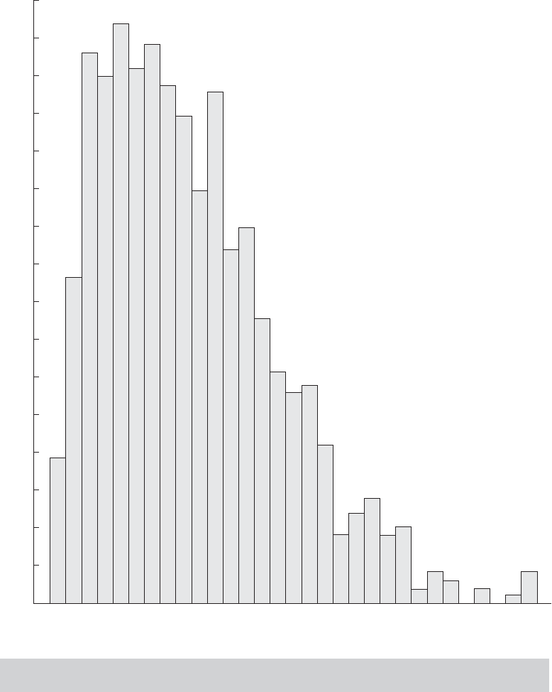
Example C.3 illustrates the behavior of the sample mean in samples of four observations

drawn from a chi-squared population with one degree of freedom. The crucial concepts illus-

trated in this example are, ﬁrst, the mean and variance results in Theorem C.1 and, second, the

phenomenon of sampling variability.

Notice that the fundamental result in Theorem C.1 does not assume a distribution for x

Indeed, looking back at Section C.3, nothing we have done so far has required any assumption

about a particular distribution.

Example C.3 Sampling Distribution of a Sample Mean

Figure C.3 shows a frequency plot of the means of 1,000 random samples of four observations

drawn from a chi-squared distribution with one degree of freedom, which has mean 1 and

variance 2.

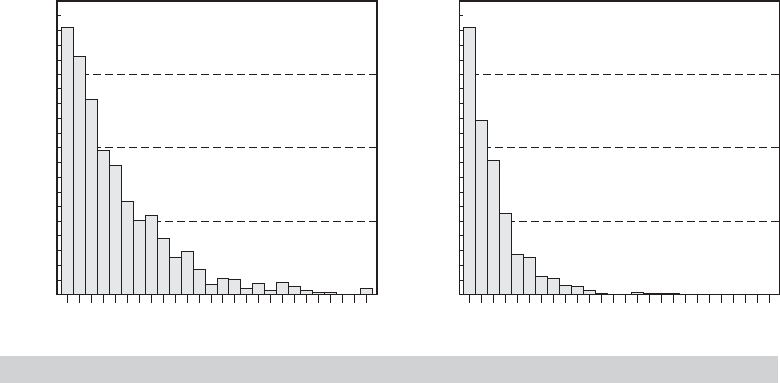
We are often interested in how a statistic behaves as the sample size increases. Example C.4

illustrates one such case. Figure C.4 shows two sampling distributions, one based on samples of

three and a second, of the same statistic, but based on samples of six. The effect of increasing

sample size in this ﬁgure is unmistakable. It is easy to visualize the behavior of this statistic if we

extrapolate the experiment in Example C.4 to samples of, say, 100.

Example C.4 Sampling Distribution of the Sample Minimum

If x

, ..., x

are a random sample from an exponential distribution with f (x) = θe

−θ x

, then the

sampling distribution of the sample minimum in a sample of n observations, denoted x

(1)

,is



(1)



= (nθ)e

−(nθ) x

(1)

Because E [x] =1/θ and Var[x] =1/θ

, by analogy E [x

(1)

] =1/(nθ ) and Var[x

(1)

] =1/(nθ )

Thus, in increasingly larger samples, the minimum will be arbitrarily close to 0. [The

Chebychev inequality in Theorem D.2 can be used to prove this intuitively appealing result.]

Figure C.4 shows the results of a simple sampling experiment you can do to demon-

strate this effect. It requires software that will allow you to produce pseudorandom num-

bers uniformly distributed in the range zero to one and that will let you plot a histogram

and control the axes. (We used NLOGIT. This can be done with Stata, Excel, or several

other packages.) The experiment consists of drawing 1,000 sets of nine random values,

, i =1, ...1,000, j =1, ..., 9. To transform these uniform draws to exponential with pa-

rameter θ—we used θ =1.5, use the inverse probability transform—see Section E.2.3. For

an exponentially distributed variable, the transformation is z

=−(1/θ ) log( 1 − U

). We then

created z

(1)

|3 from the ﬁrst three draws and z

(1)

|6 from the other six. The two histograms

show clearly the effect on the sampling distribution of increasing sample size from just

3to6.

Sampling distributions are used to make inferences about the population. To consider a

perhaps obvious example, because the sampling distribution of the mean of a set of normally

distributed observations has mean μ, the sample mean is a natural candidate for an estimate of

μ. The observation that the sample “mimics” the population is a statement about the sampling

1054

PART VI

✦

Appendices

Frequency

Mean  0.9038

Variance  0.5637

0.2 0.4 0.6 0.8 1.0 1.2 1.4 1.6 1.8 2.0 2.2 2.4 2.6 2.8 3.0

0.1

Sample mean

0.3 0.5 0.7 0.9 1.1 1.3 1.5 1.7 1.9 2.1 2.3 2.5 2.7 2.9 3.1

FIGURE C.3

Sampling Distribution of Means of 1,000 Samples of Size 4 from

Chi-Squared [1].

APPENDIX C

✦

Estimation and Inference

1055

200

150

100

0.000 0.186 0.371 0.557 0.743

Minimum of 3 Observations

0.929 1.114 1.300

Frequency

372

279

186

0.000 0.186 0.371 0.557 0.743

Minimum of 6 Observations

0.929 1.114 1.300

Frequency

FIGURE C.4

Histograms of the Sample Minimum of 3 and 6 Observations.

distributions of the sample statistics. Consider, for example, the sample data collected in Fig-

ure C.3. The sample mean of four observations clearly has a sampling distribution, which appears

to have a mean roughly equal to the population mean. Our theory of parameter estimation departs

from this point.

C.5 POINT ESTIMATION OF PARAMETERS

Our objective is to use the sample data to infer the value of a parameter or set of parameters,

which we denote θ .Apoint estimate is a statistic computed from a sample that gives a single value

for θ .Thestandard error of the estimate is the standard deviation of the sampling distribution

of the statistic; the square of this quantity is the sampling variance. An interval estimate is a

range of values that will contain the true parameter with a preassigned probability. There will be

a connection between the two types of estimates; generally, if

θ is the point estimate, then the

interval estimate will be

θ± a measure of sampling error.

An estimator is a rule or strategy for using the data to estimate the parameter. It is deﬁned

before the data are drawn. Obviously, some estimators are better than others. To take a simple ex-

ample, your intuition should convince you that the sample mean would be a better estimator of the

population mean than the sample minimum; the minimum is almost certain to underestimate the

mean. Nonetheless, the minimum is not entirely without virtue; it is easy to compute, which is oc-

casionally a relevant criterion. The search for good estimators constitutes much of econometrics.

Estimators are compared on the basis of a variety of attributes. Finite sample properties of estima-

tors are those attributes that can be compared regardless of the sample size. Some estimation prob-

lems involve characteristics that are not known in ﬁnite samples. In these instances, estimators are

compared on the basis on their large sample, or asymptotic properties. We consider these in turn.

C.5.1 ESTIMATION IN A FINITE SAMPLE

The following are some ﬁnite sample estimation criteria for estimating a single parameter. The ex-

tensions to the multiparameter case are direct. We shall consider them in passing where necessary.

1056

PART VI

✦

Appendices

DEFINITION C.2

Unbiased Estimator

An estimator of a parameter θ is unbiased if the mean of its sampling distribution is θ .

Formally,

E [

θ] = θ

E [

θ − θ] = Bias[

θ |θ ] = 0

implies that

θ is unbiased. Note that this implies that the expected sampling error is zero.

If θ is a vector of parameters, then the estimator is unbiased if the expected value of every

element of

θ equals the corresponding element of θ .

If samples of size n are drawn repeatedly and

θ is computed for each one, then the average

value of these estimates will tend to equal θ. For example, the average of the 1,000 sample means

underlying Figure C.2 is 0.9038, which is reasonably close to the population mean of one. The

sample minimum is clearly a biased estimator of the mean; it will almost always underestimate

the mean, so it will do so on average as well.

Unbiasedness is a desirable attribute, but it is rarely used by itself as an estimation criterion.

One reason is that there are many unbiased estimators that are poor uses of the data. For example,

in a sample of size n, the ﬁrst observation drawn is an unbiased estimator of the mean that clearly

wastes a great deal of information. A second criterion used to choose among unbiased estimators

is efﬁciency.

DEFINITION C.3

Efﬁcient Unbiased Estimator

An unbiased estimator

is more ef ﬁcient than another unbiased estimator

if the sam-

pling variance of

is less than that of

. That is,

Var[

] < Var[

In the multiparameter case, the comparison is based on the covariance matrices of the two

estimators;

is more efﬁcient than

if Var[

] −Var[

] is a positive deﬁnite matrix.

By this criterion, the sample mean is obviously to be preferred to the ﬁrst observation as an

estimator of the population mean. If σ

is the population variance, then

Var[x

] = σ

> Var[ ¯x] =

In discussing efﬁciency, we have restricted the discussion to unbiased estimators. Clearly,

there are biased estimators that have smaller variances than the unbiased ones we have consid-

ered. Any constant has a variance of zero. Of course, using a constant as an estimator is not likely

to be an effective use of the sample data. Focusing on unbiasedness may still preclude a tolerably

biased estimator with a much smaller variance, however. A criterion that recognizes this possible

tradeoff is the mean squared error.

APPENDIX C

✦

Estimation and Inference

1057

DEFINITION C.4

Mean Squared Error

The mean squared error of an estimator is

MSE[

θ |θ ] = E [(

θ − θ)

]

= Var[

θ] +



Bias[

θ |θ ]



if θ is a scalar,

MSE[

θ |θ ] = Var[

θ] +Bias[

θ |θ ]Bias[

θ |θ ]



if θ is a vector.

(C-9)

Figure C.5 illustrates the effect. In this example, on average, the biased estimator will be

closer to the true parameter than will the unbiased estimator.

Which of these criteria should be used in a given situation depends on the particulars of that

setting and our objectives in the study. Unfortunately, the MSE criterion is rarely operational;

minimum mean squared error estimators, when they exist at all, usually depend on unknown

parameters. Thus, we are usually less demanding. A commonly used criterion is minimum variance

unbiasedness.

Example C.5 Mean Squared Error of the Sample Variance

In sampling from a normal distribution, the most frequently used estimator for σ



i =1

( x

− ¯x )

n − 1

It is straightforward to show that s

is unbiased, so

Var [s

] =

2σ

n − 1

= MSE[s

|σ

FIGURE C.5

Sampling Distributions.

Estimator

Density

␪

unbiased ␪

biased ␪

1058

PART VI

✦

Appendices

[A proof is based on the distribution of the idempotent quadratic form (x − iμ)



(x − iμ),

which we discussed in Section B11.4.] A less frequently used estimator is

ˆσ



i =1

( x

− ¯x )

= [(n − 1) /n]s

This estimator is slightly biased downward:

E[ˆσ

] =

(n − 1) E( s

)

(n − 1) σ

so its bias is

E[ˆσ

− σ

] = Bias[ ˆσ

|σ

] =

−1

But it has a smaller variance than s

Var [ ˆσ

] =



n − 1





2σ

n − 1



< Var [s

To compare the two estimators, we can use the difference in their mean squared errors:

MSE[ ˆσ

|σ

] − MSE[s

|σ

] = σ



2n − 1

−

n − 1



< 0.

The biased estimator is a bit more precise. The difference will be negligible in a large sample,

but, for example, it is about 1.2 percent in a sample of 16.

C.5.2 EFFICIENT UNBIASED ESTIMATION

In a random sample of n observations, the density of each observation is f (x

,θ). Because the n

observations are independent, their joint density is

f (x

, x

,...,x

,θ) = f (x

,θ)f (x

,θ)··· f (x

,θ)

i=1

f (x

,θ) = L(θ |x

, x

,...,x

(C-10)

This function, denoted L(θ |X), is called the likelihood function for θ given the data X.Itis

frequently abbreviated to L(θ ). Where no ambiguity can arise, we shall abbreviate it further

to L.

Example C.6 Likelihood Functions for Exponential

and Normal Distributions

If x

, ..., x

are a sample of n observations from an exponential distribution with parameter

θ, then

L( θ) =

i =1

θe

−θ x

= θ

−θ



i =1

If x

, ..., x

are a sample of n observations from a normal distribution with mean μ and

standard deviation σ , then

L( μ, σ ) =

i =1

(2πσ

)

−1/2

−[1/(2σ

)](x

−μ)

= (2πσ

)

−n/2

−[1/(2σ

)]

( x

−μ)

(C-11)