Greene W.H. Econometric Analysis

Подождите немного. Документ загружается.

APPENDIX C

✦

Estimation and Inference

1059

The likelihood function is the cornerstone for most of our theory of parameter estimation. An

important result for efﬁcient estimation is the following.

THEOREM C.2

Cram

er–Rao Lower Bound

Assuming that the density of x satisﬁes certain regularity conditions, the variance of an

unbiased estimator of a parameter θ will always be at least as large as

[I(θ )]

−1



−E



∂

ln L(θ)

∂θ



−1







∂ ln L(θ)

∂θ





−1

. (C-12)

The quantity I(θ) is the information number for the sample. We will prove the result that the

negative of the expected second derivative equals the expected square of the ﬁrst derivative in

Chapter 14. Proof of the main result of the theorem is quite involved. See, for example,

Stuart and Ord (1989).

The regularity conditions are technical in nature. (See Section 14.4.1.) Loosely, they are

conditions imposed on the density of the random variable that appears in the likelihood function;

these conditions will ensure that the Lindeberg–Levy central limit theorem will apply to moments

of the sample of observations on the random vector y = ∂ ln f (x

|θ)/∂θ, i = 1,...,n. Among

the conditions are ﬁnite moments of x up to order 3. An additional condition normally included

in the set is that the range of the random variable be independent of the parameters.

In some cases, the second derivative of the log likelihood is a constant, so the Cram ´er–

Rao bound is simple to obtain. For instance, in sampling from an exponential distribution, from

Example C.6,

ln L = n ln θ − θ



i=1

∂ ln L

∂θ

−



i=1

so ∂

ln L/∂θ

=−n/θ

and the variance bound is [I(θ)]

−1

= θ

/n. In many situations, the second

derivative is a random variable with a distribution of its own. The following examples show two

such cases.

Example C.7 Variance Bound for the Poisson Distribution

For the Poisson distribution,

f ( x) =

−θ

ln L =−nθ +





i =1



ln θ −



i =1

ln( x

!),

∂ ln L

∂θ

=−n +



i =1

∂

ln L

∂θ

−



i =1

1060

PART VI

✦

Appendices

The sum of n identical Poisson variables has a Poisson distribution with parameter equal

to n times the parameter of the individual variables. Therefore, the actual distribution of the

ﬁrst derivative will be that of a linear function of a Poisson distributed variable. Because



i =1

] = nE [x

] = nθ, the variance bound for the Poisson distribution is [I (θ )]

−1

= θ/n.

(Note also that the same result implies that E [∂ ln L/∂θ ] = 0, which is a result we will use in

Chapter 14. The same result holds for the exponential distribution.)

Consider, ﬁnally, a multivariate case. If θ is a vector of parameters, then I(θ) is the information

matrix. The Cram ´er–Rao theorem states that the difference between the covariance matrix of

any unbiased estimator and the inverse of the information matrix,

[I(θ)]

−1



−E



∂

ln L(θ)

∂θ ∂θ





−1





∂ ln L(θ)

∂θ



∂ ln L(θ)

∂θ





−1

, (C-13)

will be a nonnegative deﬁnite matrix.

In many settings, numerous estimators are available for the parameters of a distribution.

The usefulness of the Cram´er–Rao bound is that if one of these is known to attain the variance

bound, then there is no need to consider any other to seek a more efﬁcient estimator. Regarding

the use of the variance bound, we emphasize that if an unbiased estimator attains it, then that

estimator is efﬁcient. If a given estimator does not attain the variance bound, however, then we

do not know, except in a few special cases, whether this estimator is efﬁcient or not. It may be

that no unbiased estimator can attain the Cram´er–Rao bound, which can leave the question of

whether a given unbiased estimator is efﬁcient or not unanswered.

We note, ﬁnally, that in some cases we further restrict the set of estimators to linear functions

of the data.

DEFINITION C.5

Minimum Variance Linear Unbiased

Estimator (MVLUE)

An estimator is the minimum variance linear unbiased estimator or best linear unbiased

estimator (BLUE) if it is a linear function of the data and has minimum variance among

linear unbiased estimators.

In a few instances, such as the normal mean, there will be an efﬁcient linear unbiased estima-

tor; ¯x is efﬁcient among all unbiased estimators, both linear and nonlinear. In other cases, such

as the normal variance, there is no linear unbiased estimator. This criterion is useful because we

can sometimes ﬁnd an MVLUE without having to specify the distribution at all. Thus, by limiting

ourselves to a somewhat restricted class of estimators, we free ourselves from having to assume

a particular distribution.

C.6 INTERVAL ESTIMATION

Regardless of the properties of an estimator, the estimate obtained will vary from sample to

sample, and there is some probability that it will be quite erroneous. A point estimate will not

provide any information on the likely range of error. The logic behind an interval estimate is

that we use the sample data to construct an interval, [lower (X), upper (X)], such that we can

expect this interval to contain the true parameter in some speciﬁed proportion of samples, or

APPENDIX C

✦

Estimation and Inference

1061

equivalently, with some desired level of conﬁdence. Clearly, the wider the interval, the more

conﬁdent we can be that it will, in any given sample, contain the parameter being estimated.

The theory of interval estimation is based on a pivotal quantity, which is a function of both the

parameter and a point estimate that has a known distribution. Consider the following examples.

Example C.8 Conﬁdence Intervals for the Normal Mean

In sampling from a normal distribution with mean μ and standard deviation σ ,

z =

√

n(¯x − μ)

∼ t[n − 1],

and

c =

(n − 1) s

∼ χ

[n − 1].

Given the pivotal quantity, we can make probability statements about events involving the

parameter and the estimate. Let p( g, θ ) be the constructed random variable, for example, z

or c. Given a prespeciﬁed conﬁdence level, 1 − α, we can state that

Prob(lower ≤ p( g, θ) ≤ upper) = 1 − α, (C-14)

where lower and upper are obtained from the appropriate table. This statement is then ma-

nipulated to make equivalent statements about the endpoints of the intervals. For example,

the following statements are equivalent:

Prob



−z ≤

√

n(¯x − μ)

≤ z



= 1 − α,

Prob



¯x −

√

≤ μ ≤ ¯x +

√



= 1 − α.

The second of these is a statement about the interval, not the parameter; that is, it is the

interval that is random, not the parameter. We attach a probability, or 100( 1 − α) percent

conﬁdence level, to the interval itself; in repeated sampling, an interval constructed in this

fashion will contain the true parameter 100(1 − α) percent of the time.

In general, the interval constructed by this method will be of the form

lower(X) =

θ − e

upper(X) =

θ + e

where X is the sample data, e

and e

are sampling errors, and

θ is a point estimate of θ. It is clear

from the preceding example that if the sampling distribution of the pivotal quantity is either t or

standard normal, which will be true in the vast majority of cases we encounter in practice, then

the conﬁdence interval will be

θ ± C

1−α/2

[se(

θ)], (C-15)

where se(.) is the (known or estimated) standard error of the parameter estimate and C

1−α/2

the value from the t or standard normal distribution that is exceeded with probability 1 − α/2.

The usual values for α are 0.10, 0.05, or 0.01. The theory does not prescribe exactly how to

choose the endpoints for the conﬁdence interval. An obvious criterion is to minimize the width

of the interval. If the sampling distribution is symmetric, then the symmetric interval is the

best one. If the sampling distribution is not symmetric, however, then this procedure will not be

optimal.

1062

PART VI

✦

Appendices

Example C.9 Estimated Conﬁdence Intervals for a Normal Mean

and Variance

In a sample of 25, ¯x = 1.63 and s = 0.51. Construct a 95 percent conﬁdence interval for μ.

Assuming that the sample of 25 is from a normal distribution,

Prob



−2.064 ≤

5( ¯x − μ)

≤ 2.064



= 0.95,

where 2.064 is the critical value from a t distribution with 24 degrees of freedom. Thus, the

conﬁdence interval is 1.63 ± [2.064( 0.51)/5] or [1.4195, 1.8405].

Remark: Had the parent distribution not been speciﬁed, it would have been natural to use the

standard normal distribution instead, perhaps relying on the central limit theorem. But a sam-

ple size of 25 is small enough that the more conservative t distribution might still be preferable.

The chi-squared distribution is used to construct a conﬁdence interval for the variance

of a normal distribution. Using the data from Example C.9, we ﬁnd that the usual procedure

would use

Prob



12.4 ≤

24s

≤ 39.4



= 0.95,

where 12.4 and 39.4 are the 0.025 and 0.975 cutoff points from the chi-squared (24) distribu-

tion. This procedure leads to the 95 percent conﬁdence interval [0.1581, 0.5032]. By making

use of the asymmetry of the distribution, a narrower interval can be constructed. Allocating

4 percent to the left-hand tail and 1 percent to the right instead of 2.5 percent to each, the two

cutoff points are 13.4 and 42.9, and the resulting 95 percent conﬁdence interval is [0.1455,

0.4659].

Finally, the conﬁdence interval can be manipulated to obtain a conﬁdence interval for

a function of a parameter. For example, based on the preceding, a 95 percent conﬁdence

interval for σ would be [

√

0.1581,

√

0.5032] = [0.3976, 0.7094].

C.7 HYPOTHESIS TESTING

The second major group of statistical inference procedures is hypothesis tests. The classical testing

procedures are based on constructing a statistic from a random sample that will enable the

analyst to decide, with reasonable conﬁdence, whether or not the data in the sample would

have been generated by a hypothesized population. The formal procedure involves a statement

of the hypothesis, usually in terms of a “null” or maintained hypothesis and an “alternative,”

conventionally denoted H

and H

, respectively. The procedure itself is a rule, stated in terms

of the data, that dictates whether the null hypothesis should be rejected or not. For example,

the hypothesis might state a parameter is equal to a speciﬁed value. The decision rule might

state that the hypothesis should be rejected if a sample estimate of that parameter is too far

away from that value (where “far” remains to be deﬁned). The classical, or Neyman–Pearson,

methodology involves partitioning the sample space into two regions. If the observed data (i.e.,

the test statistic) fall in the rejection region (sometimes called the critical region), then the null

hypothesis is rejected; if they fall in the acceptance region, then it is not.

C.7.1 CLASSICAL TESTING PROCEDURES

Since the sample is random, the test statistic, however deﬁned, is also random. The same test

procedure can lead to different conclusions in different samples. As such, there are two ways

such a procedure can be in error:

1. Type I error. The procedure may lead to rejection of the null hypothesis when it is true.

2. Type II error. The procedure may fail to reject the null hypothesis when it is false.

APPENDIX C

✦

Estimation and Inference

1063

To continue the previous example, there is some probability that the estimate of the parameter

will be quite far from the hypothesized value, even if the hypothesis is true. This outcome might

cause a type I error.

DEFINITION C.6

Size of a Test

The probability of a type I error is the size of the test. This is conventionally denoted α and

is also called the signiﬁcance level.

The size of the test is under the control of the analyst. It can be changed just by changing

the decision rule. Indeed, the type I error could be eliminated altogether just by making the

rejection region very small, but this would come at a cost. By eliminating the probability of a

type I error—that is, by making it unlikely that the hypothesis is rejected—we must increase the

probability of a type II error. Ideally, we would like both probabilities to be as small as possible.

It is clear, however, that there is a tradeoff between the two. The best we can hope for is that for

a given probability of type I error, the procedure we choose will have as small a probability of

type II error as possible.

DEFINITION C.7

PowerofaTest

The power of a test is the probability that it will correctly lead to rejection of a false null

hypothesis:

power = 1 −β = 1 −Prob(type II error). (C-16)

For a given signiﬁcance level α, we would like β to be as small as possible. Because β is

deﬁned in terms of the alternative hypothesis, it depends on the value of the parameter.

Example C.10 Testing a Hypothesis About a Mean

For testing H

: μ = μ

in a normal distribution with known variance σ

, the decision rule is

to reject the hypothesis if the absolute value of the z statistic,

√

n(¯x − μ

)/σ, exceeds the

predetermined critical value. For a test at the 5 percent signiﬁcance level, we set the critical

value at 1.96. The power of the test, therefore, is the probability that the absolute value of

the test statistic will exceed 1.96 given that the true value of μ is, in fact, not μ

. This value

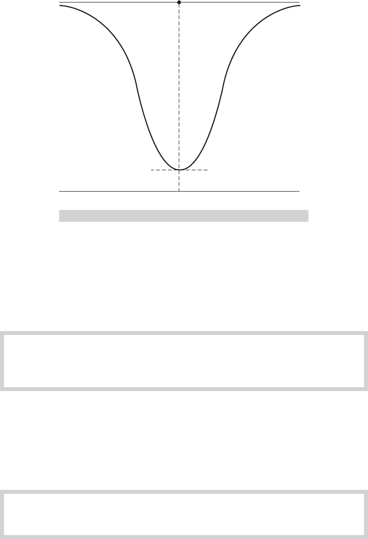
depends on the alternative value of μ, as shown in Figure C.6. Notice that for this test the

power is equal to the size at the point where μ equals μ

. As might be expected, the test

becomes more powerful the farther the true mean is from the hypothesized value.

Testing procedures, like estimators, can be compared using a number of criteria.

DEFINITION C.8

Most Powerful Test

A test is most powerful if it has greater power than any other test of the same size.

1064

PART VI

✦

Appendices

1.0

1  ␤

␣

␮

FIGURE C.6

Power Function for a Test.

This requirement is very strong. Because the power depends on the alternative hypothesis, we

might require that the test be uniformly most powerful (UMP), that is, have greater power than

any other test of the same size for all admissible values of the parameter. Thereare few situations in

which a UMP test is available. We usually must be less stringent in our requirements. Nonetheless,

the criteria for comparing hypothesis testing procedures are generally based on their respective

power functions. A common and very modest requirement is that the test be unbiased.

DEFINITION C.9

Unbiased Test

A test is unbiased if its power (1 − β) is greater than or equal to its size α for all values of

the parameter.

If a test is biased, then, for some values of the parameter, we are more likely to accept the

null hypothesis when it is false than when it is true.

The use of the term unbiased here is unrelated to the concept of an unbiased estimator.

Fortunately, there is little chance of confusion. Tests and estimators are clearly connected, how-

ever. The following criterion derives, in general, from the corresponding attribute of a parameter

estimate.

DEFINITION C.10

Consistent Test

A test is consistent if its power goes to one as the sample size grows to inﬁnity.

APPENDIX C

✦

Estimation and Inference

1065

Example C.11 Consistent Test About a Mean

A conﬁdence interval for the mean of a normal distribution is ¯x ± t

1−α/2

(s/

√

n) , where ¯x and

s are the usual consistent estimators for μ and σ (see Section D.2.1), n is the sample size,

and t

1−α/2

is the correct critical value from the t distribution with n − 1 degrees of freedom.

For testing H

: μ = μ

versus H

: μ = μ

, let the procedure be to reject H

if the conﬁdence

interval does not contain μ

. Because ¯x is consistent for μ, one can discern if H

is false as

n →∞, with probability 1, because ¯x will be arbitrarily close to the true μ. Therefore, this

test is consistent.

As a general rule, a test will be consistent if it is based on a consistent estimator of the

parameter.

C.7.2 TESTS BASED ON CONFIDENCE INTERVALS

There is an obvious link between interval estimation and the sorts of hypothesis tests we have

been discussing here. The conﬁdence interval gives a range of plausible values for the parameter.

Therefore, it stands to reason that if a hypothesized value of the parameter does not fall in this

range of plausible values, then the data are not consistent with the hypothesis, and it should be

rejected. Consider, then, testing

: θ = θ

: θ = θ

We form a conﬁdence interval based on

θ as described earlier:

θ − C

1−α/2

[se(

θ)] <θ <

θ + C

1−α/2

[se(

θ)].

is rejected if θ

exceeds the upper limit or is less than the lower limit. Equivalently, H

rejected if

θ − θ

se(

θ)

> C

1−α/2

In words, the hypothesis is rejected if the estimate is too far from θ

, where the distance is measured

in standard error units. The critical value is taken from the t or standard normal distribution,

whichever is appropriate.

Example C.12 Testing a Hypothesis About a Mean with

a Conﬁdence Interval

For the results in Example C.8, test H

: μ = 1.98 versus H

: μ = 1.98, assuming sampling

from a normal distribution:

t =

¯x − 1.98

√

1.63 − 1.98

0.102

= 3.43.

The 95 percent critical value for t(24) is 2.064. Therefore, reject H

. If the critical value for

the standard normal table of 1.96 is used instead, then the same result is obtained.

If the test is one-sided, as in

: θ ≥ θ

: θ<θ

then the critical region must be adjusted. Thus, for this test, H

will be rejected if a point estimate

of θ falls sufﬁciently below θ

. (Tests can usually be set up by departing from the decision criterion,

“What sample results are inconsistent with the hypothesis?”)

1066

PART VI

✦

Appendices

Example C.13 One-Sided Test About a Mean

A sample of 25 from a normal distribution yields ¯x = 1.63 and s = 0.51. Test

: μ ≤ 1.5,

: μ>1.5.

Clearly, no observed ¯x less than or equal to 1.5 will lead to rejection of H

. Using the borderline

value of 1.5 for μ, we obtain

Prob



√

n(¯x − 1.5)

5(1.63 − 1.5)

0.51



= Prob(t

> 1.27).

This is approximately 0.11. This value is not unlikely by the usual standards. Hence, at a

signiﬁcant level of 0.11, we would not reject the hypothesis.

C.7.3 SPECIFICATION TESTS

The hypothesis testing procedures just described are known as “classical” testing procedures. In

each case, the null hypothesis tested came in the form of a restriction on the alternative. You

can verify that in each application we examined, the parameter space assumed under the null

hypothesis is a subspace of that described by the alternative. For that reason, the models implied

are said to be “nested.” The null hypothesis is contained within the alternative. This approach

sufﬁces for most of the testing situations encountered in practice, but there are common situations

in which two competing models cannot be viewed in these terms. For example, consider a case

in which there are two completely different, competing theories to explain the same observed

data. Many models for censoring and truncation discussed in Chapter 19 rest upon a fragile

assumption of normality, for example. Testing of this nature requires a different approach from the

classical procedures discussed here. These are discussed at various points throughout the book, for

example, in Chapter 19, where we study the difference between ﬁxed and random effects models.

APPENDIX D

LARGE-SAMPLE DISTRIBUTION

THEORY

D.1 INTRODUCTION

Most of this book is about parameter estimation. In studying that subject, we will usually be

interested in determining how best to use the observed data when choosing among competing

estimators. That, in turn, requires us to examine the sampling behavior of estimators. In a few

cases, such as those presented in Appendix C and the least squares estimator considered in

Chapter 4, we can make broad statements about sampling distributions that will apply regardless

of the size of the sample. But, in most situations, it will only be possible to make approximate

statements about estimators, such as whether they improve as the sample size increases and what

can be said about their sampling distributions in large samples as an approximation to the ﬁnite

APPENDIX D

✦

Large-Sample Distribution Theory

1067

samples we actually observe. This appendix will collect most of the formal, fundamental theorems

and results needed for this analysis. A few additional results will be developed in the discussion

of time-series analysis later in the book.

D.2 LARGE-SAMPLE DISTRIBUTION THEORY

In most cases, whether an estimator is exactly unbiased or what its exact sampling variance is in

samples of a given size will be unknown. But we may be able to obtain approximate results about

the behavior of the distribution of an estimator as the sample becomes large. For example, it is

well known that the distribution of the mean of a sample tends to approximate normality as the

sample size grows, regardless of the distribution of the individual observations. Knowledge about

the limiting behavior of the distribution of an estimator can be used to infer an approximate

distribution for the estimator in a ﬁnite sample. To describe how this is done, it is necessary, ﬁrst,

to present some results on convergence of random variables.

D.2.1 CONVERGENCE IN PROBABILITY

Limiting arguments in this discussion will be with respect to the sample size n. Let x

be a sequence

random variable indexed by the sample size.

DEFINITION D.1

Convergence in Probability

The random variable x

converges in probability to a constant c if lim

n→∞

Prob(|x

−c| >

ε) = 0 for any positive ε.

Convergence in probability implies that the values that the variable may take that are not

close to c become increasingly unlikely as n increases. To consider one example, suppose that the

random variable x

takes two values, zero and n, with probabilities 1 −(1/n) and (1/n), respec-

tively. As n increases, the second point will become ever more remote from any constant but, at the

same time, will become increasingly less probable. In this example, x

converges in probability

to zero. The crux of this form of convergence is that all the mass of the probability distribution

becomes concentrated at points close to c.Ifx

converges in probability to c, then we write

plim x

= c. (D-1)

We will make frequent use of a special case of convergence in probability, convergence in mean

square or convergence in quadratic mean.

THEOREM D.1

Convergence in Quadratic Mean

If x

has mean μ

and variance σ

such that the ordinary limits of μ

and σ

are c and 0,

respectively, then x

converges in mean square to c, and

plim x

= c.

A comprehensive summary of many results in large-sample theory appears in White (2001). The results

discussed here will apply to samples of independent observations. Time-series cases in which observations

are correlated are analyzed in Chapters 20 through 23.

1068

PART VI

✦

Appendices

A proof of Theorem D.1 can be based on another useful theorem.

THEOREM D.2

Chebychev’s Inequality

If x

is a random variable and c and ε are constants, then Prob(|x

− c|>ε)≤

E[(x

− c)

]/ε

To establish the Chebychev inequality, we use another result [see Goldberger (1991, p. 31)].

THEOREM D.3

Markov’s Inequality

If y

is a nonnegative random variable and δ is a positive constant, then

Prob[y

≥ δ] ≤ E[y

]/δ.

Proof: E[y

] =Prob[y

<δ]E[y

| y

<δ] +Prob[y

≥δ]E[y

| y

≥ δ]. Because y

is non-

negative, both terms must be nonnegative, so E[y

] ≥Prob[y

≥δ]E[y

| y

≥δ].

Because E[y

| y

≥δ] must be greater than or equal to δ,E[y

] ≥Prob[y

≥δ]δ, which

is the result.

Now, to prove Theorem D.1, let y

be (x

− c)

and δ be ε

in Theorem D.3. Then, (x

− c)

>δ

implies that |x

− c| >ε. Finally, we will use a special case of the Chebychev inequality, where

c = μ

, so that we have

Prob(|x

− μ

| >ε)≤ σ

/ε

. (D-2)

Taking the limits of μ

and σ

in (D-2), we see that if

lim

n→∞

E[x

] = c, and lim

n→∞

Var[x

] = 0, (D-3)

then

plim x

= c.

We have shown that convergence in mean square implies convergence in probability. Mean-

square convergence implies that the distribution of x

collapses to a spike at plim x

, as shown in

Figure D.1.

Example D.1 Mean Square Convergence of the Sample Minimum

in Exponential Sampling

As noted in Example C.4, in sampling of n observations from an exponential distribution, for

the sample minimum x

(1)

lim

n→∞



(1)



= lim

n→∞

nθ

= 0

and

lim

n→∞

Var



(1)



= lim

n→∞

(nθ)

= 0.

Therefore,

plim x

(1)

= 0.

Note, in particular, that the variance is divided by n

. Thus, this estimator converges very

rapidly to 0.