Greene W.H. Econometric Analysis

Подождите немного. Документ загружается.

APPENDIX E

✦

Computation and Optimization

1089

DEFINITION D.15

Order less than n

A sequence c

, is of order less than n

, denoted o(n

), if and only if plim(1/n

equals

zero.

Thus, in our examples, γ

is O(n

−1

), Var[x

(1),n

]isO(n

−2

) and o(n

−1

), S

is O(n

)(δ equals +2in

this case), ln L(θ ) is O(n)(δ equals +1), and c

is O(1)(δ = 0). Important particular cases that we

will encounter repeatedly in our work are sequences for which δ =1or−1.

The notion of order of a sequence is often of interest in econometrics in the context of the

variance of an estimator. Thus, we see in Section D.3 that an important element of our strategy for

forming an asymptotic distribution is that the variance of the limiting distribution of

√

n( ¯x

−μ)/σ

is O(1). In Example D.10 the variance of m

is the sum of three terms that are O(n

−1

), O(n

−2

and O(n

−3

). The sum is O(n

−1

), because n Var[m

] converges to μ

− σ

, the numerator of the

ﬁrst, or leading term, whereas the second and third terms converge to zero. This term is also the

dominant term of the sequence. Finally, consider the two divergent examples in the preceding list.

is simply a deterministic function of n that explodes. However, ln L(θ) = n ln θ − θ

is the

sum of a constant that is O(n) and a random variable with variance equal to n/θ. The random

variable “diverges” in the sense that its variance grows without bound as n increases.

APPENDIX E

COMPUTATION AND

OPTIMIZATION

E.1 INTRODUCTION

The computation of empirical estimates by econometricians involves using digital computers

and software written either by the researchers themselves or by others.

It is also a surprisingly

balanced mix of art and science. It is important for software users to be aware of how results

are obtained, not only to understand routine computations, but also to be able to explain the

occasional strange and contradictory results that do arise. This appendix will describe some of the

basic elements of computing and a number of tools that are used by econometricians.

Section E.2

It is one of the interesting aspects of the development of econometric methodology that the adoption of

certain classes of techniques has proceeded in discrete jumps with the development of software. Noteworthy

examples include the appearance, both around 1970, of G. K. Joreskog’s LISREL [Joreskog and Sorbom

(1981)] program, which spawned a still-growing industry in linear structural modeling, and TSP [Hall (1982)],

which was among the ﬁrst computer programs to accept symbolic representations of econometric models and

which provided a signiﬁcant advance in econometric practice with its LSQ procedure for systems of equations.

An extensive survey of the evolution of econometric software is given in Renfro (2007).

This discussion is not intended to teach the reader how to write computer programs. For those who expect

to do so, there are whole libraries of useful sources. Three very useful works are Kennedy and Gentle (1980),

Abramovitz and Stegun (1971), and especially Press et al. (1986). The third of these provides a wealth of

expertly written programs and a large amount of information about how to do computation efﬁciently and

accurately. A recent survey of many areas of computation is Judd (1998).

1090

PART VI

✦

Appendices

then describes some techniques for computing certain integrals and derivatives that are recurrent

in econometric applications. Section E.3 presents methods of optimization of functions. Some

examples are given in Section E.4.

E.2 COMPUTATION IN ECONOMETRICS

This section will discuss some methods of computing integrals that appear frequently in econo-

metrics.

E.2.1 COMPUTING INTEGRALS

One advantage of computers is their ability rapidly to compute approximations to complex func-

tions such as logs and exponents. The basic functions, such as these, trigonometric functions, and

so forth, are standard parts of the libraries of programs that accompany all scientiﬁc computing

installations.

But one of the very common applications that often requires some high-level cre-

ativity by econometricians is the evaluation of integrals that do not have simple closed forms and

that do not typically exist in “system libraries.” We will consider several of these in this section.

We will not go into detail on the nuts and bolts of how to compute integrals with a computer;

rather, we will turn directly to the most common applications in econometrics.

E.2.2 THE STANDARD NORMAL CUMULATIVE

DISTRIBUTION FUNCTION

The standard normal cumulative distribution function (cdf) is ubiquitous in econometric models.

Yet this most homely of applications must be computed by approximation. There are a number

of ways to do so.

Recall that what we desire is

(x) =

−∞

φ(t) dt, where φ(t) =

√

2π

−t

One way to proceed is to use a Taylor series:

(x) ≈



i=0

(x

)

(x − x

)

The normal cdf has some advantages for this approach. First, the derivatives are simple and not

integrals. Second, the function is analytic; as M −→ ∞ , the approximation converges to the true

value. Third, the derivatives have a simple form; they are the Hermite polynomials and they can

be computed by a simple recursion. The 0th term in the preceding expansion is (x) evaluated

at the expansion point. The ﬁrst derivative of the cdf is the pdf, so the terms from 2 onward are

the derivatives of φ(x), once again evaluated at x

. The derivatives of the standard normal pdf

obey the recursion

/φ(x) =−xφ

i−1

/φ(x) − (i − 1)φ

i−2

/φ(x),

where φ

is d

φ(x)/dx

. The zero and one terms in the sequence are one and −x. The next term

is x

− 1, followed by 3x − x

and x

− 6x

+ 3, and so on. The approximation can be made

Of course, at some level, these must have been programmed as approximations by someone.

Many system libraries provide a related function, the error function, erf(x) = (2/

√

π)

−t

dt. If this is

available, then the normal cdf can be obtained from (x) =

erf(x/

√

2), x ≥0 and (x) =1−(−x), x ≤0.

APPENDIX E

✦

Computation and Optimization

1091

2.00

0.20

0.00

0.20

0.40

0.60

0.80

1.00

1.20

1.50 1.00 0.50 0.00

0.50 1.00 1.50 2.00

F 

FA 

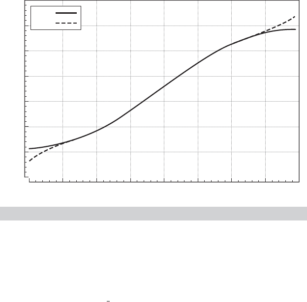
FIGURE E.1

Approximation to Normal cdf.

more accurate by adding terms. Consider using a ﬁfth-order Taylor series approximation around

the point x =0, where (0) =0.5 and φ(0) =0.3989423. Evaluating the derivatives at zero and

assembling the terms produces the approximation

(x) ≈

+ 0.3989423[x − x

/6 + x

/40].

[Some of the terms (every other one, in fact) will conveniently drop out.] Figure E.1 shows the

actual values (F ) and approximate values (FA) over the range −2 to 2. The ﬁgure shows two

important points. First, the approximation is remarkably good over most of the range. Second, as

is usually true for Taylor series approximations, the quality of the approximation deteriorates as

one gets far from the expansion point.

Unfortunately, it is the tail areas of the standard normal distribution that are usually of

interest, so the preceding is likely to be problematic. An alternative approach that is used much

more often is a polynomial approximation reported by Abramovitz and Stegun (1971, p. 932):

(−|x|) = φ(x)



i=1

+ ε(x), where t = 1/[1 + a

|x|].

(The complement is taken if x is positive.) The error of approximation is less than ±7.5 × 10

−8

for all x. (Note that the error exceeds the function value at |x| > 5.7, so this is the operational

limit of this approximation.)

E.2.3 THE GAMMA AND RELATED FUNCTIONS

The standard normal cdf is probably the most common application of numerical integration of a

function in econometrics. Another very common application is the class of gamma functions. For

1092

PART VI

✦

Appendices

positive constant P, the gamma function is

(P) =

∞

P−1

−t

dt.

The gamma function obeys the recursion (P) = (P − 1)( P − 1), so for integer values of

P,(P) =(P −1)! This result suggests that the gamma function can be viewed as a generalization

of the factorial function for noninteger values. Another convenient value is (

) =

√

π.By

making a change of variable, it can be shown that for positive constants a, c, and P,

∞

P−1

−at

dt =

∞

−(P+1)

−a/t

dt =





−P/c







. (E-1)

As a generalization of the factorial function, the gamma function will usually overﬂow for

the sorts of values of P that normally appear in applications. The log of the function should

normally be used instead. The function ln (P) can be approximated remarkably accurately with

only a handful of terms and is very easy to program. A number of approximations appear in the

literature; they are generally modiﬁcations of Stirling’s approximation to the factorial function

P! ≈ (2π P)

1/2

−P

,so

ln (P) ≈ (P − 0.5)ln P − P + 0.5ln(2π) + C + ε(P),

where C is the correction term [see, e.g., Abramovitz and Stegun (1971, p. 257), Press et al. (1986,

p. 157), or Rao (1973, p. 59)] and ε(P) is the approximation error.

The derivatives of the gamma function are

(P)

∞

(ln t)

P−1

−t

dt.

The ﬁrst two derivatives of ln (P) are denoted (P) = 



/ and 



(P) = (



− 

2

)/ 

and

are known as the digamma and trigamma functions.

The beta function, denoted β(a, b),

β(a, b) =

a−1

(1 −t)

b−1

dt =

(a)(b)

(a + b)

is related.

E.2.4 APPROXIMATING INTEGRALS BY QUADRATURE

The digamma and trigamma functions, and the gamma function for noninteger values of P and

values that are not integers plus

, do not exist in closed form and must be approximated. Most

other applications will also involve integrals for which no simple computing function exists. The

simplest approach to approximating

F(x) =

U(x)

L(x)

f (t) dt

For example, one widely used formula is C = z

−1

/12 − z

−3

/360 − z

−5

/1260 + z

−7

/1680 − q, where z = P

and q = 0ifP > 18, or z = P + J and q = ln[P( P + 1)(P + 2) ···(P + J − 1)], where J = 18 − INT(P),if

not. Note, in the approximation, we write (P) = (P!)/P + a correction.

Tables of speciﬁc values for the gamma, digamma, and trigamma functions appear in Abramovitz and Stegun

(1971). Most contemporary econometric programs have built-in functions for these common integrals, so the

tables are not generally needed.

APPENDIX E

✦

Computation and Optimization

1093

is likely to be a variant of Simpson’s rule, or the trapezoid rule. For example, one approximation

[see Press et al. (1986, p. 108)] is

F(x) ≈ 



+···+

N−2

N−1



where f

is the function evaluated at N equally spaced points in [L, U] including the endpoints

and  = (L −U)/(N −1). There are a number of problems with this method, most notably that

it is difﬁcult to obtain satisfactory accuracy with a moderate number of points.

Gaussian quadrature is a popular method of computing integrals. The general approach is

to use an approximation of the form

W(x) f (x) dx ≈



j=1

f (a

where W(x) is viewed as a “weighting” function for integrating f (x), w

is the quadrature weight,

and a

is the quadrature abscissa. Different weights and abscissas have been derived for several

weighting functions. Two weighting functions common in econometrics are

W(x) = x

−x

, x ∈ [0, ∞),

for which the computation is called Gauss–Laguerre quadrature, and

W(x) = e

−x

, x ∈ (−∞, ∞),

for which the computation is called Gauss–Hermite quadrature. The theory for deriving weights

and abscissas is given in Press et al. (1986, pp. 121–125). Tables of weights and abscissas for many

values of M are given by Abramovitz and Stegun (1971). Applications of the technique appear

in Chapters 14 and 17.

E.3 OPTIMIZATION

Nonlinear optimization (e.g., maximizing log-likelihood functions) is an intriguing practical prob-

lem. Theory provides few hard and fast rules, and there are relatively few cases in which it is

obvious how to proceed. This section introduces some of the terminology and underlying theory

of nonlinear optimization.

We begin with a general discussion on how to search for a solution

to a nonlinear optimization problem and describe some speciﬁc commonly used methods. We

then consider some practical problems that arise in optimization. An example is given in the ﬁnal

section.

Consider maximizing the quadratic function

F(θ) = a + b



θ −



Cθ,

where C is a positive deﬁnite matrix. The ﬁrst-order condition for a maximum is

∂ F(θ)

∂θ

= b − Cθ = 0. (E-2)

This set of linear equations has the unique solution

θ = C

−1

b. (E-3)

There are numerous excellent references that offer a more complete exposition. Among these are Quandt

(1983), Bazaraa and Shetty (1979), Fletcher (1980), and Judd (1998).

1094

PART VI

✦

Appendices

This is a linear optimization problem. Note that it has a closed-form solution; for any a, b, and C,

the solution can be computed directly.

In the more typical situation,

∂ F(θ)

∂θ

= 0 (E-4)

is a set of nonlinear equations that cannot be solved explicitly for θ.

The techniques considered

in this section provide systematic means of searching for a solution.

We now consider the general problem of maximizing a function of several variables:

maximize

F(θ), (E-5)

where F(θ) may be a log-likelihood or some other function. Minimization of F(θ) is handled by

maximizing −F(θ). Two special cases are

F(θ) =



i=1

(θ), (E-6)

which is typical for maximum likelihood problems, and the least squares problem,

(θ) =−(y

− f (x

, θ))

. (E-7)

We treated the nonlinear least squares problem in detail in Chapter 7. An obvious way to search

for the θ that maximizes F(θ) is by trial and error. If θ has only a single element and it is known

approximately where the optimum will be found, then a grid search will be a feasible strategy. An

example is a common time-series problem in which a one-dimensional search for a correlation

coefﬁcient is made in the interval (−1, 1). The grid search can proceed in the obvious fashion—

that is, ...,−0.1, 0, 0.1, 0.2,...,then

max

−0.1to

max

+0.1 in increments of 0.01, and so on—until

the desired precision is achieved.

If θ contains more than one parameter, then a grid search

is likely to be extremely costly, particularly if little is known about the parameter vector at the

outset. Nonetheless, relatively efﬁcient methods have been devised. Quandt (1983) and Fletcher

(1980) contain further details.

There are also systematic, derivative-free methods of searching for a function optimum that

resemble in some respects the algorithms that we will examine in the next section. The downhill

simplex (and other simplex) methods

have been found to be very fast and effective for some

problems. A recent entry in the econometrics literature is the method of simulated annealing.

These derivative-free methods, particularly the latter, are often very effective in problems with

many variables in the objective function, but they usually require far more function evaluations

than the methods based on derivatives that are considered below. Because the problems typically

analyzed in econometrics involve relatively few parameters but often quite complex functions

involving large numbers of terms in a summation, on balance, the gradient methods are usually

going to be preferable.

Notice that the constant a is irrelevant to the solution. Many maximum likelihood problems are presented

with the preface “neglecting an irrelevant constant.” For example, the log-likelihood for the normal linear

regression model contains a term—(n/2) ln(2π)—that can be discarded.

See, for example, the normal equations for the nonlinear least squares estimators of Chapter 7.

Least squares is, of course, a minimization problem. The negative of the criterion is used to maintain

consistency with the general formulation.

There are more efﬁcient methods of carrying out a one-dimensional search, for example, the golden section

method. See Press et al. (1986, Chap. 10).

See Nelder and Mead (1965) and Press et al. (1986).

See Goffe, Ferrier, and Rodgers (1994) and Press et al. (1986, pp. 326–334).

Goffe, Ferrier, and Rodgers (1994) did ﬁnd that the method of simulated annealing was quite adept at

ﬁnding the best among multiple solutions. This problem is common for derivative-based methods, because

they usually have no method of distinguishing between a local optimum and a global one.

APPENDIX E

✦

Computation and Optimization

1095

E.3.1 ALGORITHMS

A more effective means of solving most nonlinear maximization problems is by an iterative

algorithm:

Beginning from initial value θ

, at entry to iteration t,ifθ

is not the optimal value for

θ, compute direction vector 

, step size λ

, then

t+1

= θ

+ λ



. (E-8)

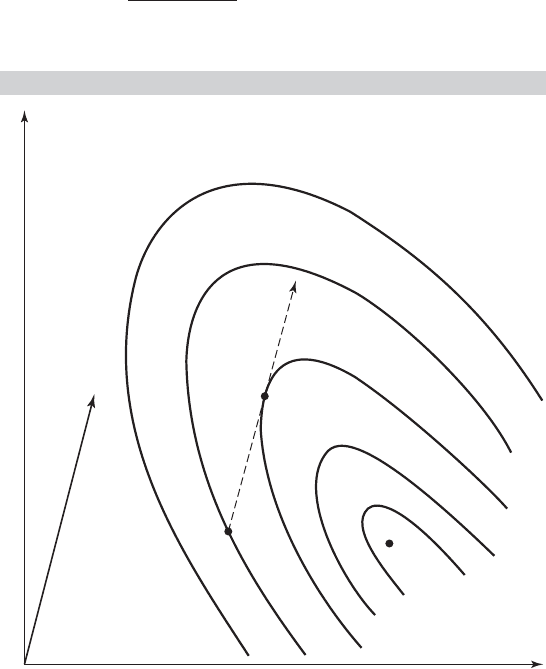
Figure E.2 illustrates the structure of an iteration for a hypothetical function of two variables.

The direction vector 

is shown in the ﬁgure with θ

. The dashed line is the set of points θ



. Different values of λ

lead to different contours; for this θ

and 

, the best value of λ

about 0.5.

Notice in Figure E.2 that for a given direction vector 

and current parameter vector θ

a secondary optimization is required to ﬁnd the best λ

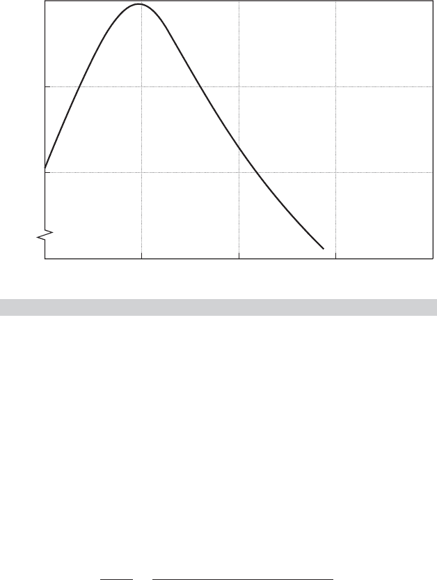
. Translating from Figure E.2, we obtain

the form of this problem as shown in Figure E.3. This subsidiary search is called a line search, as

we search along the line θ

+ λ



for the optimal value of F(.). The formal solution to the line

search problem would be the λ

that satisﬁes

∂ F(θ

+ λ



)

∂λ

= g(θ

+ λ



)





= 0, (E-9)

FIGURE E.2

Iteration.

1.8

1.9

2.0

2.1

2.2

2.3

␪



␪

1096

PART VI

✦

Appendices

1.9

1.95

2.0

0.5

F(␪

 ␭



)

1 1.5

␭

FIGURE E.3

Line Search.

where g is the vector of partial derivatives of F(.) evaluated at θ

+λ



. In general, this problem

will also be a nonlinear one. In most cases, adding a formal search for λ

will be too expensive,

as well as unnecessary. Some approximate or ad hoc method will usually be chosen. It is worth

emphasizing that ﬁnding the λ

that maximizes F (θ

+λ



) at a given iteration does not generally

lead to the overall solution in that iteration. This situation is clear in Figure E.3, where the optimal

value of λ

leads to F(.) = 2.0, at which point we reenter the iteration.

E.3.2 COMPUTING DERIVATIVES

For certain functions, the programming of derivatives may be quite difﬁcult. Numeric approx-

imations can be used, although it should be borne in mind that analytic derivatives obtained

by formally differentiating the functions involved are to be preferred. First derivatives can be

approximated by using

∂ F(θ)

∂θ

≈

F(···θ

+ ε ···) − F(···θ

− ε ···)

2ε

The choice of ε is a remaining problem. Extensive discussion may be found in Quandt (1983).

There are three drawbacks to this means of computing derivatives compared with using

the analytic derivatives. A possible major consideration is that it may substantially increase the

amount of computation needed to obtain a function and its gradient. In particular, K +1 function

evaluations (the criterion and K derivatives) are replaced with 2K + 1 functions. The latter may

be more burdensome than the former, depending on the complexity of the partial derivatives

compared with the function itself. The comparison will depend on the application. But in most

settings, careful programming that avoids superﬂuous or redundant calculation can make the

advantage of the analytic derivatives substantial. Second, the choice of ε can be problematic. If

it is chosen too large, then the approximation will be inaccurate. If it is chosen too small, then

there may be insufﬁcient variation in the function to produce a good estimate of the derivative.

APPENDIX E

✦

Computation and Optimization

1097

A compromise that is likely to be effective is to compute ε

separately for each parameter, as in

= Max[α|θ

|,γ]

[see Goldfeld and Quandt (1971)]. The values α and γ should be relatively small, such as 10

−5

Third, although numeric derivatives computed in this fashion are likely to be reasonably accurate,

in a sum of a large number of terms, say, several thousand, enough approximation error can accu-

mulate to cause the numerical derivatives to differ signiﬁcantly from their analytic counterparts.

Second derivatives can also be computed numerically. In addition to the preceding problems,

however, it is generally not possible to ensure negative deﬁniteness of a Hessian computed in

this manner. Unless the choice of ε is made extremely carefully, an indeﬁnite matrix is a possi-

bility. In general, the use of numeric derivatives should be avoided if the analytic derivatives are

available.

E.3.3 GRADIENT METHODS

The most commonly used algorithms are gradient methods, in which



= W

, (E-10)

where W

is a positive deﬁnite matrix and g

is the gradient of F(θ

= g(θ

) =

∂ F(θ

)

∂θ

. (E-11)

These methods are motivated partly by the following. Consider a linear Taylor series approxima-

tion to F(θ

+ λ



) around λ

= 0:

F(θ

+ λ



)  F(θ

) + λ

g(θ

)





. (E-12)

Let F(θ

+ λ



) equal F

t+1

. Then,

t+1

− F

 λ





If 

= W

, then

t+1

− F

 λ



If g

is not 0 and λ

is small enough, then F

t+1

− F

must be positive. Thus, if F(θ) is not already

at its maximum, then we can always ﬁnd a step size such that a gradient-type iteration will lead

to an increase in the function. (Recall that W

is assumed to be positive deﬁnite.)

In the following, we will omit the iteration index t, except where it is necessary to distinguish

one vector from another. The following are some commonly used algorithms.

Steepest Ascent The simplest algorithm to employ is the steepest ascent method, which uses

W = I so that  = g. (E-13)

As its name implies, the direction is the one of greatest increase of F (.). Another virtue is that

the line search has a straightforward solution; at least near the maximum, the optimal λ is

λ =

−g



, (E-14)

A more extensive catalog may be found in Judge et al. (1985, Appendix B). Those mentioned here are some

of the more commonly used ones and are chosen primarily because they illustrate many of the important

aspects of nonlinear optimization.

1098

PART VI

✦

Appendices

where

H =

∂

F(θ)

∂θ ∂θ



Therefore, the steepest ascent iteration is

t+1

= θ

−



. (E-15)

Computation of the second derivatives matrix may be extremely burdensome. Also, if H

is not

negative deﬁnite, which is likely if θ

is far from the maximum, the iteration may diverge. A

systematic line search can bypass this problem. This algorithm usually converges very slowly,

however, so other techniques are usually used.

Newton’s Method The template for most gradient methods in common use is Newton’s

method. The basis for Newton’s method is a linear Taylor series approximation. Expanding the

ﬁrst-order conditions,

∂ F(θ)

∂θ

= 0,

equation by equation, in a linear Taylor series around an arbitrary θ

yields

∂ F(θ)

∂θ

 g

+ H

(θ − θ

) = 0, (E-16)

where the superscript indicates that the term is evaluated at θ

. Solving for θ and then equating

θ to θ

t+1

and θ

to θ

, we obtain the iteration

t+1

= θ

− H

−1

. (E-17)

Thus, for Newton’s method,

W =−H

−1

,  =−H

−1

g,λ= 1. (E-18)

Newton’s method will converge very rapidly in many problems. If the function is quadratic, then

this method will reach the optimum in one iteration from any starting point. If the criterion

function is globally concave, as it is in a number of problems that we shall examine in this text,

then it is probably the best algorithm available. This method is very well suited to maximum

likelihood estimation.

Alternatives to Newton’s Method Newton’s method is very effective in some settings, but it

can perform very poorly in others. If the function is not approximately quadratic or if the current

estimate is very far from the maximum, then it can cause wide swings in the estimates and even

fail to converge at all. A number of algorithms have been devised to improve upon Newton’s

method. An obvious one is to include a line search at each iteration rather than use λ = 1. Two

problems remain, however. At points distant from the optimum, the second derivatives matrix

may not be negative deﬁnite, and, in any event, the computational burden of computing H may be

excessive.

The quadratic hill-climbing method proposed by Goldfeld, Quandt, and Trotter (1966) deals

directly with the ﬁrst of these problems. In any iteration, if H is not negative deﬁnite, then it is

replaced with

= H −αI, (E-19)