Graebel W.P. Advanced Fluid Mechanics
Подождите немного. Документ загружается.

314 Multidimensional Computational Methods
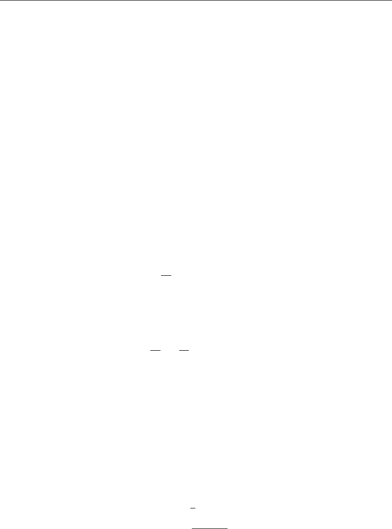
12.11 Cloud in Cell Method (CIC)
This method is a variation on the discrete vortex method and was first introduced by
Christiansen (1973). Instead of tracking individual vortices as in DVM, a grid is placed
on the region, and as a vortex moves within a sector of the grid, its vorticity is distributed
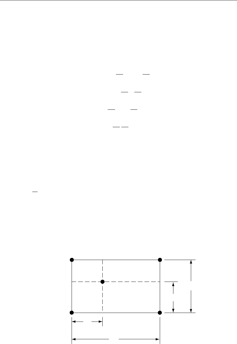
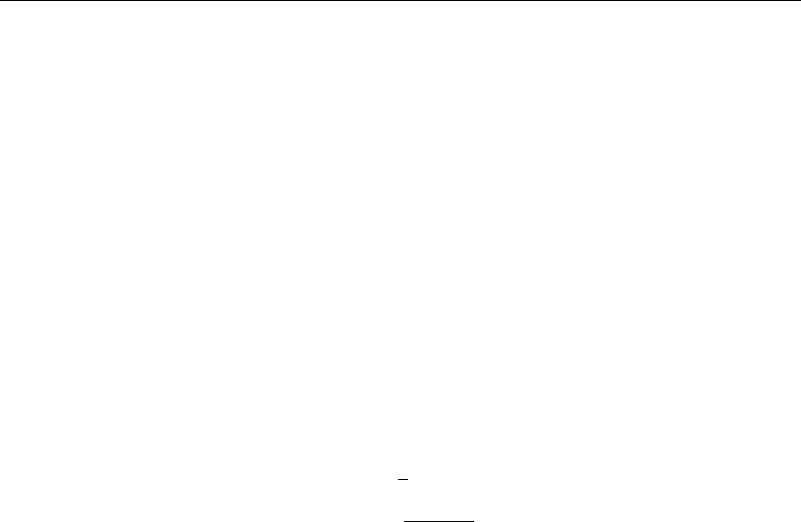
to the corners of the sector. (See Figure 12.11.1.) For a sector x by y, if the vortex
is at a location !x !y with respect to the corner of the sector, the vorticity " might
be distributed to the corners according to
"
ij
=
1−
!x
x
1−
!y
y
" =A
1
"
"
ij+1
=
1−
!x
x
!y
y
" =A
2
"
"
i+1j
=
!x
x
1−
!y
y
" =A
3
"
"
i+1j+1
=
!x
x
!y
y
" =A
4
"
(12.11.1)
After this distribution, the stream function can be solved from
2
=" (12.11.2)
The induced velocities and positions for finding how fast the vortex travels are then
found from
d
dt
x
n
y
n
=
u
n
v
n
=A
1
u
v
ij
+A
2
u
v
i+1j
+A
3
u
v
ij+1
+A
4
u
v
i+1j+1
(12.11.3)
For 1,000 vortices the CIC method appears to be about 20 times faster than the DVM
method. More references to this method and its implementation can be found in Roberts
and Christiansen (1972), Milinazzo and Saffman (1977), Chorin (1978), Alexandrou
(1986), and Hong (1988).
(i, j )
(i
+ 1, j )
(i
+ 1, j + 1)
(i, j
+ 1)
ω
δ
x
δy
Δ x
Δ y
Figure 12.11.1 Computational molecule for the cloud-in-cell method
Problems—Chapter 12 315
Problems—Chapter 12
In the following problems use either the program languages specified in the text or a
spreadsheet.
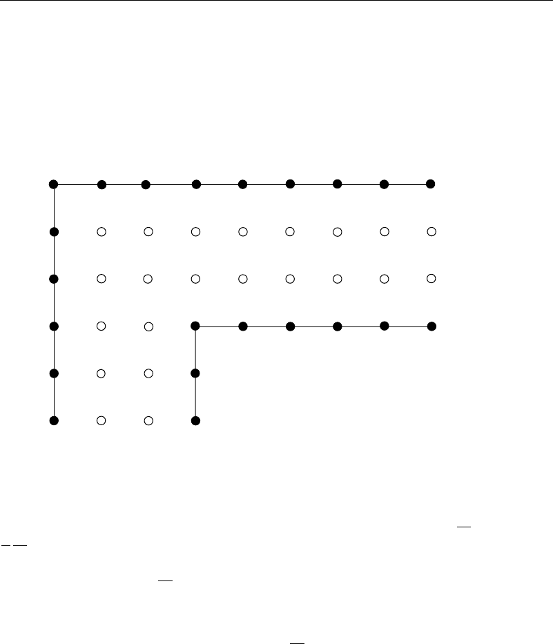
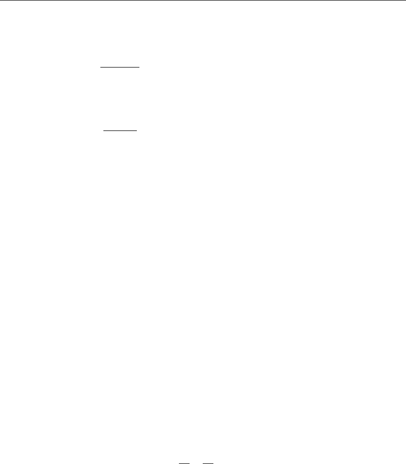
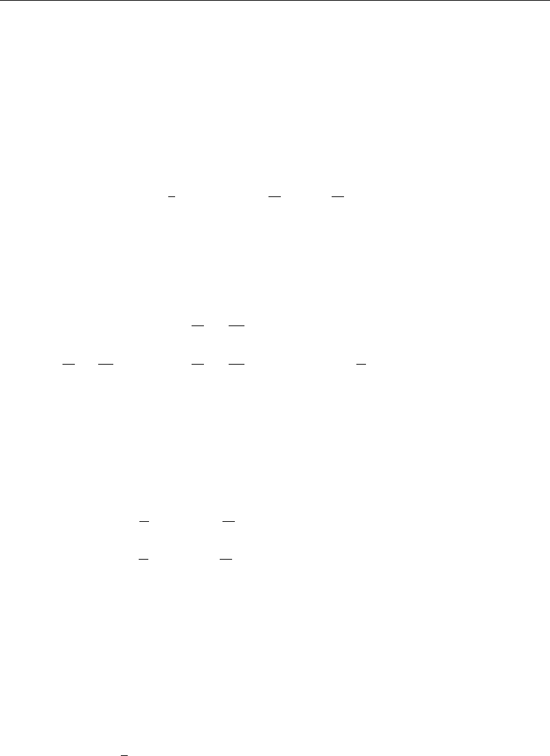
12.1 Use simple relaxation (equation (12.2.1a)) to find the values on the center line
of the elbow. On the inner boundary of the el (filled dots) the value is 0, on the outer
boundary it is 1, and the end points 1 and 10 average the two boundary values. Do at
least 10 iterations.
7
22
1211
2120
109
19
8
1817
6
16
5
4
3
15
2
14
1
13
P12.1 Flow in an elbow
12.2 Repeat problem 12.1, this time using successive overrelaxation (SOR). Take
the relaxation parameter to be 1.7.
12.3 Use the leapfrog method to solve the one-dimensional wave equation
2
f
x
2
=
1
c
2
2
f
t
2
subject to the conditions
fx 0 =sin x
f
t
x 0 =0 0 ≤x ≤ 1f0t=f1t=0
To start the solution, introduce a row of fictitious grid points at t =−t, where
fx −t = fx 0 −2t
f
t
x 0
Let x = 01 and t = x/c The wave speed can be taken as unity. Compute for at
least 20 time steps.
12.4 An explicit method for the diffusion equation f/t =
2
f/x
2
is given by
fi j +1 = fi j +
fi −1j−2fi j +fi +1j
, where = t/x
2
≤ 05.
Solve this for the conditions
f0t=0f1t=1 fx 0 =
$
4x 0 ≤ x ≤04
−x +2 04 ≤ x ≤ 1
Take =025 and x =01.
316 Multidimensional Computational Methods
12.5 An implicit formula for solving the unsteady flow in a channel, given
by the parabolic equation
u
t
=−
p
x
+
2
u
y
2
,isui j −ui j − 1 =−t
p
x
+
ui −1j−2ui j +ui +1j
, where is defined by =t/x
2
. This scheme
is apparently stable for all positive values of . Solve for flow starting from rest with
u0 = u1 = 0
p
x
=
$
0t≤0
−1t>0
Take = 05x= 01t= 01, and do 200 time steps. Compare with the exact
solution (parabolic profile).
12.6 Repeat the previous problem, this time using the Crank-Nicholson method, with
the more accurate finite difference equation in the form
ui j −ui j −1 =−
t
p
x
+
1
2
ui −1j−2ui j +ui +1j
+
1
2
ui −1j−1 −2ui j −1 +ui +1j−1
12.7 Repeat problem 12.5, this time using the DuFort-Frankel method for solving the
problem. This method is explicit and uses
ui−1j−uij−1−uij+1+ui+1j
x
2
for the second
derivative in x and
uij+1−uij−1
2t
for the time derivative.
a. Put these approximations into the Navier-Stokes equation and rearrange to
obtain a form suited to solving for the velocity at the grid points.
b. Draw the computational molecule for this method. Indicate round dots where
space derivatives are taken and squares where time derivatives are taken.
12.8 For the diffusion equation in two space derivatives and one time derivative
the alternating direction implicit method (ADI) is unconditionally stable. Starting with
f
t
=
2
f
x
2
+
2
f
y
2
, the method uses the form
f
∗
i j −fi j k
t/2
=
f
∗
i +1j−2f
∗
i j +f
∗
i −1j
x
2
+
fi j +1k−2fi j k +fi j −1k
y
2
and follows it with
fi j k +1 −f
∗
i j
t/2
=
f
∗
i +1j−2f
∗
i j +f
∗
i −1j
x
2
+
fi j +1k+1 −2fi j k +1 +fi j −1k+1
y
2
The first solves for the intermediate values f
∗
, the second completing the solution for
f at the next time step. Rearrange the equations to put them into a form suitable for
programming.
12.9 One way of dealing with the nonlinearities of the Navier-Stokes equations is
to treat steady-state flows as transient flows starting from a quiescent state. For natural
Problems—Chapter 12 317
convection on a vertical semi-infinite plate, start with the boundary layer equations in
the nondimensional form
u
t
+u
u
x
+v
u
y
=T +
2
u
y
2
T
t
+u
T
x
+v
T
y
=Pr
2
T
y
2
u
x
+
v
y
=0
and write them in an explicit finite difference form. Propose a scheme for solution.
12.10 For the linear wave equation
2
u
x
2
=
1
a
2
2
u
t
2
use the method of characteristics to
solve for a disturbance moving from left to right and striking a wall at x = 0. The x
interval is in the range −0 20 ≤ x ≤0. The disturbance is initially zero except in the
interval −009 ≤ x ≤−005 and a = 343 meters/sec. Continue the calculation until the
disturbance moves out of the domain.
Appendix
A.1 Vector Differential Calculus 318
A.2 Vector Integral Calculus 320
A.3 Fourier Series and Integrals 323
A.4 Solution of Ordinary Differential
Equations 325
A.4.1 Method of Frobenius 325
A.4.2 Mathieu Equations 326
A.4.3 Finding Eigenvalues—The
Riccati Method 327
A.5 Index Notation 329
A.6 Tensors in Cartesian Coordinates 333
A.7 Tensors in Orthogonal Curvilinear
Coordinates 337
A.7.1 Cylindrical Polar
Coordinates 339
A.7.2 Spherical Polar
Coordinates 340
A.8 Tensors in General Coordinates 341
I am very well acquainted, too, with matters mathematical,
I understand equations, both the simple and quadratical:
About binomial theorem I’m teeming with a lot of news,
With many cheerful facts about the square of the hypotenuse.
William S. Gilbert
A.1 Vector Differential Calculus
Derivatives of a vector function of the space coordinates can be performed in any
combination of the coordinate directions. A useful differentiation operator is the del
operator, denoted by the symbol , or del, defined in Cartesian coordinates as
=del = i
x
+j
y
+k
z
(A.1.1)
The operator often appears in partial differential equations in its “squared” form
2
= · =Laplacian =harmonic operator =
2
x
2
+
2
y
2
+
2
z
2
(A.1.2)
318
A.1 Vector Differential Calculus 319
To illustrate some of the uses of the del operator, consider a unit vector a with
direction cosines a
x
a
y
a
z
. Then, the operation a · acting on a vector F gives the
derivative of F in the direction of a,or
a ·F = a
x
F
x
+a
y
F
y
+a
z
F
z
The operator v · is encountered often in fluid mechanics, particularly where v is the
velocity vector. The operator itself is not a vector, since v · = ·v, and is referred to
as a pseudo-vector.
Frequent uses of the operator include its operations on a scalar and also in vector
multiplications. For instance, if is a scalar function of the coordinates, then
=grad = i
x
+j
y
+k
z
(A.1.3)
is called the gradient of . Its magnitude tells us relative information about the spacing
of lines of constant . Where the magnitude of grad is large, the constant lines are
closer together than where it is small. The direction of grad is locally normal to the
surface = constant.
The scalar quantity
·F =div F =
F
x
x
+
F
y
y
+
F
z
z
(A.1.4)
is called the divergence of F. It tells us the quantity of F that passes through a surface.
The vector quantity
×F =curl F = i
F
z
y
−
F
y
z
+j
F
x
z
−
F
z
x
+k
F
y
x
−
F
x
y
(A.1.5)
is called the curl of F and gives information on how much F is twisting or rotating. It
also tells the direction of this rotation.
Some useful formulas that involve the del operator follow. They can easily be
verified by expanding left- and right-hand sides and comparing the results.
fF =f·F+F·f
×fF = f×F+f ×F
·A×B =B· ×A −A · ×B
×A×B =B·A −A ·B+A ·B −B ·A
A·B =A·B +B ·A+A × ×B +B× ×A
×f = 0 for any scalar f
· ×F =0 for any vector F
× ×F = ·F −
2
F
B·A =
1
2
×A×B −A × ×B −B× ×A +A ·B
−A ·B +B ·A
A theorem due to Helmholtz states that any vector F can be expressed in the form
F =grad +curl A where div A =0 (A.1.6)
320 Appendix
Here, is called the scalar potential of F, and A is the vector potential of F. Since
·F =
2
(A.1.7)
and
×F =−
2
A (A.1.8)
the scalar potential represents the irrotational part of F (the “curl-less” portion of F),
and the vector potential represents the rotational portion of F.
The Helmholtz decomposition (equation (A.1.6)) results in the two Poisson equa-
tions (A.1.7) and (A.1.8) (a Poisson equation is a Laplace equation with a nonhomoge-
neous “right-hand side”). These can in principle be solved, giving
x =
V
·Fx
gx x
dV
Ax =−
V
×Fx
gx x
dV
(A.1.9)
where
gxx
=Green’s function =
⎛
⎜
⎝
1
2
ln
x −x
in two dimensions
−1
4
x −x
in three dimensions
⎞
⎟
⎠
(A.1.10)
Notice that the Green’s function is our potential for a source. The solution equation
(A.1.9), however, in general does not satisfy the constraint ·A = 0. To take care of
this, replace equation (A.1.6) by
F =grad +curl A
+grad a (A.1.11)
Since curl grad a = 0 for any a, F has not been affected in any manner. Thus, A
is
given by equation (A.1.9). Since A
+grad a now replaces A, the requirement div A =0
is replaced by divA
+grad a =0. Thus, if a is defined by
2
a =−div A
(A.1.12)
giving
a =−
V
·A
x
gx x
dV
(A.1.13)
the constraint has been satisfied. (Note: In two dimensions the indicated volume integrals
become surface integrals.)
A.2 Vector Integral Calculus
There are several interesting and useful theorems regarding the operator and integra-
tion that are useful in fluid mechanics, both in deriving the basic equations and in putting
them in a form suitable for numerical calculation. They will be listed without proof.
These theorems are all closely related, and the names Gauss, Green, and Stokes are
intimately connected with them. In their use, they are closely related to the concept of
integration by parts of elementary calculus and can be thought of as a multidimensional
extension of that concept.
A.2 Vector Integral Calculus 321
Gauss’s theorem states the following:
In three dimensions, with S a closed surface,
S
n ·
R −R
0
R −R
0
3
dS =
0ifR
0
is outside of S
4 if R
0
is inside of S
(A.2.1a)
In two dimensions, with C a closed curve,
C
n ·
r −r
0
r −r
0
2
ds =
0ifr
0
is outside of S
2 if r
0
is inside of S
(A.2.1b)
In both dimensions the integrand will be recognized as the radial velocity component
of a source located at R
0
in three dimensions and r
0
in two dimensions.
Stokes’s theorem is useful for changing line integrals to surface integrals and vice
versa. In its simplest form it is
C
t ·Fds =
S
n · ×FdS =
S
n × ·FdS (A.2.2)
where C is a closed curve bounding the surface S, n is a unit normal to the surface S,
and t is a unit tangent to the curve C. Note that C and S do not have to lie in a plane
and that C could bound an infinite number of different surfaces S.
Variations of Stokes’s theorem include the following:
C
tfds=
S
n ×f dS
C
t ×Fds =
S
n ·F −n ×FdS =
S
n ××FdS
C
t ·Fds =
S
n · ×FdS =
S
n ×·FdS
C
t ×nfds=
S
−f +nn ·f +f·ndS
with
·n =−
1
R
1
+
1
R
2
R
1
and R
2
being the principal radii of curvature of the surface S.
The divergence theorem, also called Green’s theorem, is used for transforming
surface integrals to volume integrals and is stated as
S
n ·FdS =
V
·FdV (A.2.3)
where S is a surface enclosing the volume V , and n is again the unit outward normal.
The theorem states that the net outflow of F through S is made up of the sum of the
outflows from all of the regions inside of S.
322 Appendix
Variations of this theorem include the following:
S
n ×FdS =
V
×FdV
S
n ·
FdS =
V
2
FdV
S
n ·
fdS=
V
2
f dV
S
nfdS=
V
f dV
On a surface,
S
n ××FdS =−
C
t ×Fds
S
n ·
×F
dS =
S
n ×
·FdS =
C
t·Fds
S
·FdS =
C
t ×n ·Fds
S
n ×f dS =
C
fds
From these theorems several results follow that are useful in inviscid flow theory.
Green’s first identity
S
f
h
n
dS =
V
f ·h +f
2
hdV (A.2.4)
Here f and h are any two scalar functions of the coordinates, and S is the surface
enclosing V . This identity follows from Gauss’s theorem with F =fh.
Green’s second identity
C
h
f
n
−f
h
n
dS =
V
h
2
f −f
2
hdV (A.2.5)
Here f and h are any two scalar functions of the coordinates. This identity follows
from Green’s first identity, written first as in equation (A.2.3) and again with f and h
interchanged. The result follows by taking the difference of the two.
Green’s third identity
P =−
V
gP, Q
2
(Q) dV
+
S
gP Qn ·Q −Qn ·gP QdS
(A.2.6)
where in equation (A.2.5)
gP Q =Green’s function =
⎛
⎜
⎝
1
2
ln
P −Q
for two dimensional problems
−1
4
P −Q
for three dimensional problems
⎞
⎟
⎠
(A.2.7)
Here P is the position vector of a point in the interior of V and Q is the position vector
of a dummy point of integration, on the surface for the surface integral, and in the
A.3 Fourier Series and Integrals 323
interior for the volume integral. The function g is called the Green’s function for the
Laplace operator and is seen to be the velocity potential for a source.
A.3 Fourier Series and Integrals
Many times it is useful to represent a function in terms of an infinite series of simple
functions. A classic example of this is the Fourier series, where if ft is defined over
an interval 0 ≤ t ≤ T , the Fourier series representation of ft is
ft =
1
2
a
0
+
n =1
a
n
cos
nt
T
+b
n
sin
nt
T
. (A.3.1)
This representation makes ft periodic with period T ; that is, ft +nT =ft for any
integer n.
The coefficients a
n
and b
n
are determined by the property of the trigonometric
functions that, for integers m and n,
T
0
sin
nt
T
cos
mt
T
dt =0
T
0
sin
nt
T
sin
mt
T
dt =
T
0
cos
nt
T
cos
mt
T
dt =0ifn =m
T
2
if n =m
(A.3.2)
The trigonometric functions are said to be orthogonal to one another, as the operation
of taking a product of two of them and then integrating is analogous to taking a dot
product of two vectors.
To use the orthogonality property, multiply both sides of equation (A.3.1) by either
the sine or cosine of mt/T , and then integrate over the period T . Interchanging
integration and summation, the result is
a
n
=
2
T
T
0
ft cos
nt
T
dt
b
n
=
2
T
T
0
ft sin
nt
T
dt for n =0 1 2
(A.3.3)
If the function ft is discontinuous at either a point interior to, or at either
end of, the interval, the series will converge to the average value at that point. Near
the discontinuity, the series sum will show oscillations and overshoots, the Gibbs
phenomenon.
The Fourier series representation of a function as given by equations (A.3.1) and
(A.3.3) is sometimes also called the finite Fourier transform. By DeMoivre’s theorem,
the sines and cosines can be replaced by exponentials so that the Fourier series (equation
(A.3.1)) becomes
ft =
1
2
a
0
+
n =1
a
n
−ib
n
e
int/T
+
n =1
a
n
+ib
n
e
−int/T
=
n =−
c
n
e
int/T