Graebel W.P. Advanced Fluid Mechanics
Подождите немного. Документ загружается.

304 Multidimensional Computational Methods
Thus, by doing the numerical solution twice with different step sizes, the solution
represented by equation (12.4.28) has an extra order of accuracy.
12.4.7 Further Choices for Dealing with Nonlinearities
What makes solution techniques in computational fluid mechanics unique is how they
deal with the convective acceleration terms u
u
x
+v
u
y
. There are a number of different
ways to do this.
1. Lagging computation. Evaluate u, v at their old position. Then
u
u
x
+v
u
y
≈u
nj
u
n+1j
−u
nj
x
+v
nj
u
nj+1
−u
nj
y
(12.4.29)
This is first order in the “marching coordinate” x and will cause trouble when x
derivatives become large.
2. Simple iterative update. Use the lagging computation, and then repeat the compu-
tation using equation (12.4.29) but with the newly computed u
n+1j
. The process
can be repeated several times.
3. Newton linearization. The convergence of a method is improved if the continuity
and momentum equations are solved in a coupled manner.
4. Extrapolation of coefficients. When using u
n+1j
compute it using
u
n+1j
=u
nj
+
u
x
x
n
y
j
x where
u
x
x
n
y
j
=
u
nj
−u
n−1j
x
(12.4.30)
12.4.8 Upwind Differencing for Convective Acceleration Terms
Perhaps the most popular method for improving calculation of convective terms is that
of upwind differencing. Traditional methods for calculating Lf =
f
t
+u
f
x
use
Lf ≈
f
n+1j
−f
nj
t
+u
f
nj+1
−f
nj
x
(12.4.31)
In upwind differencing, provided u is positive, instead use
Lf ≈
f
n+1j
−f
nj
t
+u
f
nj
−f
nj−1
x
(12.4.32)
Comparing these two equations shows that the only change has been in the x differen-
cing, which is now in the upwind direction rather than the current (downwind) direction.
The effect of this change is to introduce an artificial viscosity into the problem so that
if we were trying to solve Lf = 0, using upwind differencing we would actually be
solving
f
t
=
uf
x
+
artificial
2
f
x
2
+higher-order terms and differences.
The artificial viscosity is given by
artificial
=
1
2
u
x −ut
. Providing this artificial
viscosity is positive, the use of upwind differencing is necessary for stability of the
computations.
12.5 Multistep, or Alternating Direction, Methods 305
12.5 Multistep, or Alternating Direction, Methods
12.5.1 Alternating Direction Explicit (ADE) Method
Consider the differential equation
f
t
=
2
f
x
2
=
x
f
x
(12.5.1)
Since in the previous section we saw that it was advantageous at times to take derivatives
in different ways, one suggestion for approximating equation (12.5.1) is
f
n+1j
−f
nj
t
=
f
nj+1
−f
nj
−
f
n+1j
−f
n+1j−1
x
2
(12.5.2)
Solving for updated values gives
f
n+1j
=
1−
1+
f
nj
+
1+
f
nj+1
+
1+
f
n+1j−1
(12.5.3)
If we are clever enough to sweep through our equations in the direction of increasing
j, the last term on the right-hand side is known, and we have a simple explicit method.
The good news is that, for equation (12.5.1), this method is unconditionally stable,
with errors of second order in both t and x. The bad news is that, if convection terms
are added to equation (12.5.1), the method may be unconditionally unstable.
12.5.2 Alternating Direction Implicit (ADI) Method
As our starting point we will be more ambitious than in the previous section, dealing
with one time dimension and two space directions. For our model equation let
f
t
=−u
f
x
−v
f
y
+
2
f
x
2
+
2
f
y
2
(12.5.4)
To do our time differencing proceed in two steps:
Step1
f
n+1/2
−f
n
t/2
=−u
f
n+1/2
x
−v
f
n
y
+
2
f
n+1/2
x
2
+
2
f
n
y
2
(12.5.5)
Step2
f
n+1
−f
n
t/2
=−u
f
n+1/2
x
−v
f
n+1
y
+
2
f
n+1/2
x
2
+
2
f
n+1
y
2
(12.5.6)
Notice that although each of the two steps are implicit, the resulting equations are
tridiagonal and thus easy to solve. The error is second order in each of the three
incremental deltas.
Formally, this method has unconditional stability. However, it can become unstable
if too big a time step is used. This is especially true if the boundary conditions are
allowed to lag in time. See Roache (1976, page 92).
In equations (12.5.5) and (12.5.6) details on the x and y differencing have been
omitted. One might use
2
f
nij
x
2
≈
f
ni+1j
−2f
nij
+f
ni−1j
x
2
and
2
f
nij
y
2
≈
f
nij+1
−2f
nij
+f
nij−1
y
2
Further, to keep second-order accuracy, use u
n+1/2
v
n
in equation (12.5.5) and u
n+1/2
v
n+1
in equation (12.5.6).
306 Multidimensional Computational Methods
To use this method to solve the full Navier-Stokes equations would require an
implicit coupled solution of an equation like (12.5.4) in the stream function and another
one in vorticity, both solutions to be carried out at the two times n +1/2 and n +1.
This would be a formidable task! These two methods, wherein the differencing of space
derivatives is split into two time steps, are the first of many splitting methods which
have been introduced.
Hyperbolic Partial Differential Equations
12.6 Method of Characteristics
Early in this chapter, we briefly examined the three basic classes of partial differential
equations and saw examples. We will now examine them more generally and derive a
method suitable for solving hyperbolic differential equations.
The forms of the three equations given in equation (12.1.1) can in two dimensions
be generalized by the form
A
2
f
x
2
+2B
2
f
xy
+C
2
f
y
2
=E (12.6.1)
Here A, B, C, and E are real and may depend on f and its first derivatives. Coordinates
x and y are not necessarily space coordinates; one could also be a time dimension. Next,
ask the question, When and where are infinitesimal variations of the first derivatives of
f allowed, or alternatively, Where are first derivatives of f continuous? This question
can be phrased in terms of the solution of three equations in three unknowns—that is,
A
2
f
x
2
+2B
2
f
xy
+C
2
f
y
2
=E
dx
2
f
x
2
+dy
2
f
xy
=d
f
x
(12.6.2)
dx
2
f
xy
+dy
2
f
y
2
=d
f
y
where the second and third lines represent the differentials of the first derivatives.
Using Cramer’s rule, this system is easily solved, giving
2
f
x
2
=
N
1
D
2
f
xy
=
N
2
D
2
f
y
2
=
N
3
D
(12.6.3)
with
D =
A 2BC
dx dy 0
0 dx dy
N
1
=
E 2BC
d
f
x
dy 0
d
f
y
dx dy
N
2
=
AEC
dx d
f
x
0
0 d
f
y
dy
N
3
=
A 2BE
dx dy d
f
x
0 dx d
f
y
(12.6.4)
12.6 Method of Characteristics 307
By the usual restriction of Cramer’s rule, this is an acceptable solution except where
the denominator D vanishes. Expanding this determinant, we find it vanishes where
Ady
2
+Cdx
2
−2Bdxdy =0; that is, along the lines of slope
dy
dx
=
B ±
√
B
2
−AC
A
(12.6.5)
This pair of lines are called the characteristic lines, or just characteristics,of
equation (12.6.1). Notice the following:
1. If B
2
−AC < 0, both of the characteristics are imaginary and play no decisive
role in the solution. This is the general definition of elliptic partial differential
equations.
2. If B
2
−AC =0, there is only one real characteristic. This is the general definition
of parabolic partial differential equations.
3. If B
2
−AC > 0, both of the characteristics are real. This is the general definition
of hyperbolic partial differential equations. We will concentrate further attention
on this latter case.
If a region covered by characteristics is to have a solution, it is necessary that the
numerators in equation (12.6.3) also vanish, so l’Hospital’s rule can be used. Expanding
all three of the determinants, we find with the help of equation (12.6.5) that
N
1
=
dy
dx
2
N
3
and N
2
=−
dy
dx
N
3
(12.6.6)
so all three numerators are zero on the characteristics provided N
3
= 0, which
occurs when
d
f
y
=−
A
C
dy
dx
d
f
x
+
E
C
dy (12.6.7)
With the aid of equations (12.6.5) and (12.6.7), a solution can now be constructed.
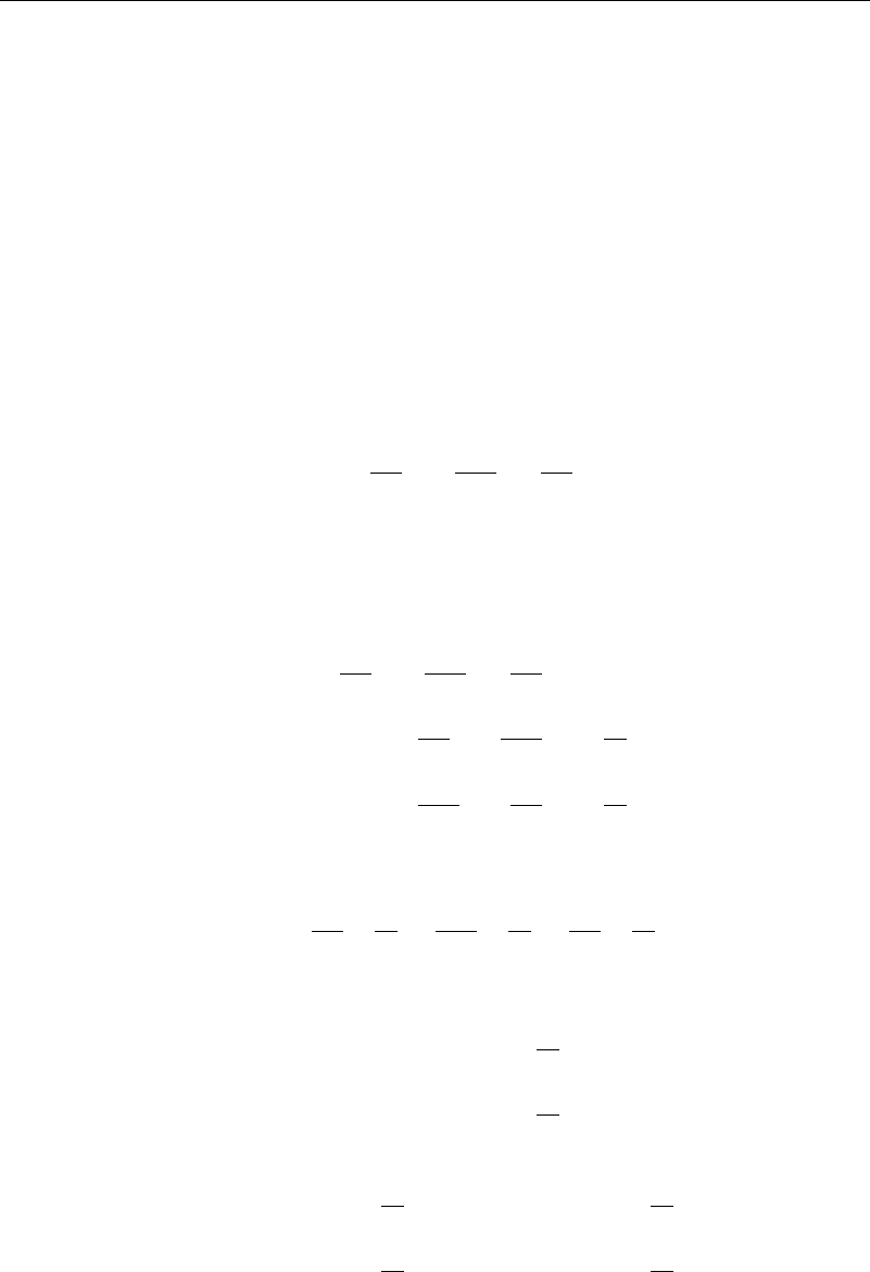
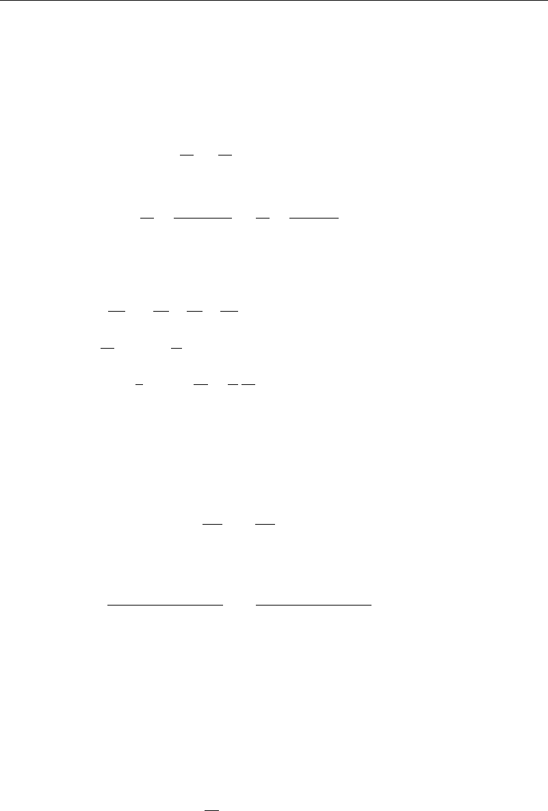
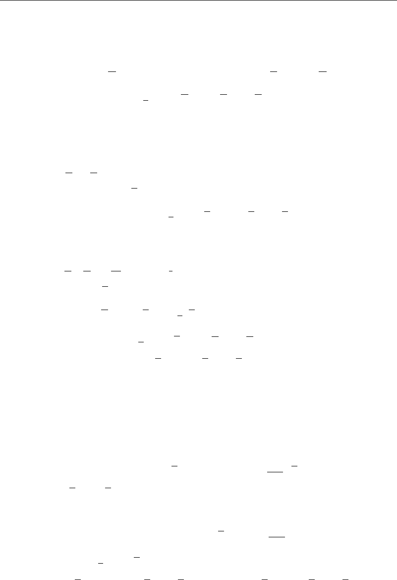
Suppose in Figure 12.6.1 that the derivatives of the function f is known on curve
1-2. Using equation (12.6.5), construct a series of characteristics on a closely spaced
number of points on this curve. Label the characteristics + if the plus sign in front of
the square root was used, and − otherwise. Notice that in the roughly triangular region
1-2-3 the + and − characteristics intersect, whereas outside this region there are no
intersections.
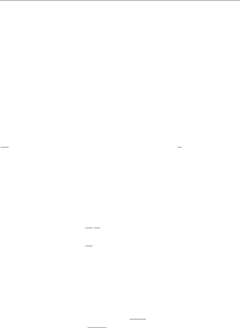
Next, magnify the small region a-b-c in Figure 12.6.1 as in Figure 12.6.2. Point c
is at the position
x
c
y
c
, determined by solving
y
c
−y
a
=
B +
√
B
2
−AC
A
a
x
c
−x
a
y
c
−y
b
=
B −
√
B
2
−AC
A
b
x
c
−x
b
(12.6.8)
Similarly, from equation (12.6.7) write
f
c
y
−
f
a
y
=−
B +
√
B
2
−AC
C
a
f
c
x
−
f
a
x
+
E
C
a
y
c
−y
a
f
c
y
−
f
b
y
=−
B −
√
B
2
−AC
C
b
f
c
x
−
f
b
x
+
E
C
b
y
c
−y
b
(12.6.9)
308 Multidimensional Computational Methods
y
x
1
3
a
b
+
+
+
+
+
+
+
+
+
+
_
_
_
_
_
_
_
_
_
_
_
c
2
Figure 12.6.1 Method of characteristics—region of solubility
(x
a
, y
a
)
(x
b
, y
b
)
(x
c
, y
c
)
Figure 12.6.2 Method of characteristics—detail of two intersecting characteristic lines
thereby solving for the derivatives of f at c. This process can be continued repeatedly
throughout the region 1-2-3, obtaining all derivatives of the function within this region.
Outside this region, no solution is possible due to insufficient data.
Note that if there is a rigid boundary (wall) or a line of symmetry, then a point
c can land on a wall and there is no − characteristic to meet it. The wall boundary
condition replaces this, however, so a solution is still possible.
In inviscid compressible isentropic flow, an equation similar to (12.6.1) governs
the flow with f the velocity potential, and
A =a
2
−u
2
B =−uv C =a
2
−v
2
a
2
=a
2
0
−
k −1
2
u
2
+v
2
(12.6.10)
u and v being the x and y velocity components (derivatives of “f”) and a the speed of
sound. Where the flow is supersonic, the equations become hyperbolic.
The method of characteristics predates computers by almost a century. If one is
analyzing or designing flow in a nozzle, it is a problem that can easily be solved
12.7 Leapfrog Method—Explicit 309
with a pencil, eraser, and adding machine. With modern computers, however, programs
using this methodology become somewhat complicated, since even if the original data
is given on a straight line, the subsequent line will more than likely be curved. Often
interpolation is used to keep a straight grid in the region of solution. Characteristics can
be lines of discontinuity of derivatives of f, but not of f itself.
Even first-order differential equations can have characteristics. If the same procedure
is pursued on the equation
u
t
+u
u
x
=fu x t (12.6.11)
for example, the result is
u
t
=
fdx −udu
dx −udt
u
x
=
du −fdt
dx −udt
(12.6.12)
The equation of the characteristic is dx =udt, and along the characteristic udu =fdx.
As an example of the use of the method of characteristics, the equations for analysis
of a water hammer are
g
H
x
+V
V
x
+
V
t
+
f
2D
V
V
=0
x
AV
+
t
A
=0 with (12.6.13)
gH =
p
+gz
t
=
K
p
t
K=bulk modulus.
The method of characteristics has been used for this problem with much success.
12.7 Leapfrog Method—Explicit
For the one-dimensional wave equation
2
f
t
2
=a
2
2
f
x
2
(12.7.1)
a method that gives interesting results is the leapfrog method. If centered differences
are used for the two second derivatives, equation (12.7.1) becomes
f
n+1j
−2f
nj
+f
n−1j
t
=a
2
f
nj+1
−2f
nj
+f
nj−1
x
(12.7.2)
Solving for f at the latest time step gives
f
n+1j
=2
1−A
2
f
nj
−f
n−1j
+A
2
f
nj+1
+f
nj−1
(12.7.3)
where A = at/x is the Courant number. Notice that when A = 1, the value at the
same position but preceding time drops out of the calculation.
The exact solution to equation (12.7.1) is known to be
fx t = Fx −at +Gx +at (12.7.4)
where F and G depend on initial conditions according to
fx 0 =Fx +Gx
f
t
x 0 =a
−F
0 +G
0
(12.7.5)
310 Multidimensional Computational Methods
Taking x
1
t
1
as a starting point and letting x
i
=x
1
+i−1x t
n
=t
1
+n−1t, then
x −at = +ix −nat =x
1
−x −at
1
−t and
x +at = +ix +nat =x
1
−x +at
1
−t
(12.7.6)
Inserting these into equation (12.7.3) with A =1 find that
−f
n−1j
+f
nj+1
+f
nj−1
=F
+i −j −1x
+G
+i +j −1x
+F
+i −j +1x
+G
+i +j +1x
−F
+i −j −1x
−G
+i +j −1x
=F
+i −j −1x
+G
+i +j +1x
=f
n+1j
(12.7.7)
Thus, for a Courant number of unity, the method gives the exact solution.
The reason for this happy result can be found by comparing the calculation procedure
with the characteristics of equation (12.7.1), which are given by
dx
dt
=±a. The slopes of
the lines connecting x
n+1j
with x
nj−1
and x
nj+1
are
x
t
=±a/A, so when the Courant
number is unity, the leapfrog method corresponds to the method of characteristics. If
we were to choose A<1, we are within the triangle of the characteristic lines, and our
computation is using valid information and the result is stable. If, however, we were to
choose A>1, we would be using information that is known not to be pertinent to the
calculation, and the calculation becomes unstable.
One drawback of the leapfrog method is that to start the calculations, there is a
need to know the solution at t
0
. To handle this, place a fictitious row at t
0
and let
f
1j
=F
x
1
−at
1
+G
x
1
+at
1
and
f
0j
=f
2j
−2a
−F
x
1
−at
1
+G
x
1
+at
1
t
(12.7.8)
Then
f
2j
=f
1j−1
+f
1j+1
−f
0j
=f
1j−1
+f
1j+1
−f
2j
+2a
−F
x
1
−at
1
+G
x
1
+at
1
t or (12.7.9)
f
2j
=
1
2
f
1j−1
+f
1j+1
+a
−F
x
1
−at
1
+G
x
1
+at
1
t
This is the starting formula for the method.
12.8 Lax-Wendroff Method—Explicit
Many of the equations of fluid mechanics are of the type
U
t
+
F
x
=0 (12.8.1)
for instance, the one-dimensional compressible flow equation where
U =
u
F =
⎛
⎝
u
u
2
2
+
a
2
k −1
⎞
⎠
(12.8.2)
12.9 MacCormacks Methods 311
The first of these equations is the continuity equation, the second the momentum
equation. The form of equation (12.8.1) is often referred to as a conservative form. The
Navier-Stokes equations and the inviscid compressible flow equations are examples that
fit this general form.
For the Lax-Wendroff method, let
F
t
=
F
U
U
t
=A
F
x
(12.8.3)
Differentiating equation (12.8.1) with respect to time yields
2
U
t
2
=−
t
F
x
=−
x
F
t
=−
x
A
F
x
(12.8.4)
From equation (12.8.2) find that
A =
⎛
⎜
⎜
⎝
F
1
U
1
F
1
U
2
F
2
U
1
F
2
U
2
⎞
⎟
⎟
⎠
=
⎛
⎝
u
2a
k −1
da
d
u
⎞
⎠
(12.8.5)
Then
U
n+1j
≈U
nj
+t
U
t
nj
+
t
2
2
2
U
t
2
nj
≈U
nj
+t
−
F
x
nj
+
t
2
2
x
A
F
x
nj
≈U
nj
−
t
2x
F
nj+1
−F
nj−1
+
t
2
2x
x
A
nj+1/2
F
nj+1/2
x
−A
nj−1/2
F
nj−1/2
x
(12.8.6)
≈U
nj
−
t
2x
F
nj+1
−F
nj−1
+
t
2
4x
2
A
nj+1
+A
nj
F
nj+1
−F
nj
−
A
nj
+A
nj−1
F
nj
−F
nj−1
This method is explicit and stable providing 0 ≤
t
x
≤1 with an error of order
1
6
t
2
3
U
t
3
+
1
6
x
2
3
U
x
3
. It is usually easy to program, although nonlinear problems require some
adjustment to the method. More details can be found in Lax (1954), Smith (1978), and
Ferziger (1981).
12.9 MacCormacks Methods
Over the years, R. W. MacCormack has investigated a series of approaches to the
conservative form (equation (12.8.1)), which have proven to be useful for computations.
Some of these methods are outlined here.
312 Multidimensional Computational Methods
12.9.1 MacCormack’s Explicit Method
This method uses a predictor-corrector approach, where an estimate of one of the
variables is first made and then updated in a later calculation. For equation (12.8.1)
MacCormack used
Predictors:
U
n+1j
=U
nj
−
F
nj+1
−F
nj
t/x
F
n+1j
=F
U
n+1j
Corrector: U
n+1j
=
1
2
U
nj
+U
n+1j
−
F
n+1j
−F
n+1j−1
t/x
(12.9.1)
the superposed bars denoting the predicted quantities.
Examples of the application of these include the following:
1. The one-dimensional wave equation
For
f
t
+a
f
x
=0, application of MacCormack’s explicit method (1969) gives
Predictor:
f
n+1j
=f
nj
−a
f
nj+1
−f
nj
t/x
Corrector: f
n+1j
=
1
2
f
nj
+f
n+1j
−a
f
n+1j
−f
n+1j−1
(12.9.2)
2. Burger’s equation
For
f
t
+
F
x
=
2
f
x
2
F=af +
1
2
bf
2
, application of MacCormack’s explicit method gives
Predictors:
f
n+1j
=f
nj
−
F
nj+1
−F
nj
t/x +r
f
nj+1
−2f
nj
+f
nj−1
F
n+1j
=af
n+1j
+
1
2
b
f
2
n+1j
Corrector: f
n+1j
=
1
2
f
nj
+f
n+1j
−
F
n+1j
−F
n+1j−1
t/x
+r
f
n+1j+1
−2f
n+1j
+f
n+1j−1
(12.9.3)
where r = t/x
2
.
12.9.2 MacCormack’s Implicit Method
In 1981 MacCormack suggested that for Burger’s equation the predictor-corrector pro-
cedure could be varied according to
Predictor
1+t/x
f
n+1j
=
f
nj
explicit
+
t
x
f
n+1j+1
where
f
n+1j
=f
n+1j
−f
nj
f
nj
explicit
=−a
f
nj+1
−f
nj
t/x +r
f
nj+1
−2f
nj
+f
nj−1
Corrector
1+t/x
f
n+1j
=
f
nj
explicit
+
t
x
f
n+1i−1
where
f
n+1j
=
1
2
f
nj
+f
n+1
j
+f
n+1j
(12.9.4)
f
nj
explicit
=−a
f
n+1j
−f
n+1j−1
t/x +r
f
n+1j+1
−2f
n+1j
+f
n+1j−1
12.10 Discrete Vortex Methods (DVM) 313
Here, is a constant such that ≥max
a +2/x −x/t 0
. This method is uncon-
ditionally stable and second-order accurate provided t/x
2
is bounded as t and
x approach zero.
12.10 Discrete Vortex Methods (DVM)
The methods previously discussed all start with an equation and then use finite differ-
ences or a similar procedure to transfer the mathematics from calculus to algebra. They
deal with flows that are well defined both physically and mathematically throughout a
region that is generally fixed. In flows that are separated, however, such as in the wake
of a bluff body, a wing, or a propellor, the portion of the flow that is of greatest interest
is in the vortices that are shed and find their way downstream. The Kármán vortex street
is an example of this.
Discrete vortex methods try to model, or simulate, these effects much in the manner
of the Kármán vortex street. Vorticity is generated at a boundary, often in the boundary
layer. At the separation point the vorticity tends to leave the boundary and move into
a flow region that is more or less inviscid. There the vorticity will move according to
D
Dt
≈ 0. The position of this bit of vorticity will change according to
dr
dt
= v, where
the velocity is a combination of the inviscid flow plus the induced velocity from all
previous bits of shed vorticity.
To make this description more specific, consider a two-dimensional flow in the
wake of a cylinder. The boundary layer flow is solved and the separation point
determined by some separation criteria such as Stratford’s. To get the vortex out
of the boundary layer, a random walk procedure can be used. Chorin (1978) sug-
gested that, to avoid the singularities in the vortexes such as discussed in the chap-
ters on inviscid flows, “vortex blobs” could be introduced, with stream functions of
the form
=
⎧
⎪
⎪
⎨
⎪
⎪
⎩
2
r
!
for
r
<!
2
ln
r
for
r
≥!
(12.10.1)
This gives constant velocity inside the vortex. The choice of the parameter ! is left up to
the user. As the blobs are released from the boundary layer, they are moved according
to the induced velocities.
There are some matters that remain, such as dealing with combining of vortices
if or when they collide, what to do when they leave the computational region, when
they reenter the boundary layer, and so forth. These can be dealt with in many ways
that fit the specific situation at hand and that deal with practical matters, such as the
capacity of the computer and time available. For instance, instead of the description
of the vortex blob just given, the formulation v =
2z−z
0
F, where F is a vorticity
modification function such as F =
99r/!
n
1+99r/!
n
nbeing an integer greater than or equal
to 2. This makes the self-induced velocity zero at the center of the blob and still
has the velocity behave as a line vortex away from the flow. More possibilities con-
cerning the implementation of this method can be found in Alexandrou (1986) and
Hong (1988).