Graebel W.P. Advanced Fluid Mechanics

Подождите немного. Документ загружается.

284 Multidimensional Computational Methods

Hyperbolic: 

V =



t

The wave equation is the most familiar form of hyperbolic equation. A propagation

velocity c is associated with the time derivative. Thus, a disturbance of an existing

condition at any point takes a finite time before its effect is noted at distant points.

Whereas solutions of the other two classes tend to be smooth, hyperbolic equations can

have abrupt discontinuities (shocks) in the solutions.

Parabolic equations are associated with diffusion processes such as heat, mass, and

concentration diffusion. There is no wave speed associated with this, so mathematically

a point an infinite distance from a place of change of conditions knows of the change

instantly. The Prandtl boundary layer equations, wherein the x second derivative term

is neglected, is frequently referred to as the parabolized Navier-Stokes equations, since

the highest order of the stream-wise derivative is one.

The elliptic type of equation, of which Laplace’s equation is the prime example,

has each location communicating at all times with all other locations in the domain,

as indicated by the mean value theorem that states that the value of the function at

the center of a circle or sphere is the average of the values on the surface. Thus, a

change at one point in the domain instantly affects every other point. Formally, the

steady-state Navier-Stokes equations belong in this class because of the order of the

viscous terms. At large Reynolds numbers, however, the magnitude of the convective

acceleration essentially overcomes this, and the behavior becomes either more like the

parabolic or hyperbolic classes.

Even for inviscid flows with free surfaces, the fact that surface and interfacial waves

can propagate at finite speeds indicates behavior more of a hyperbolic than elliptic

nature. This is brought about by the boundary conditions. So while classifications are

useful, one should keep in mind that there are other influences on the nature of the

solution.

Elliptic Partial Differential Equations

12.2 Relaxation Methods

Since the Laplace equation is perhaps the oldest and most used of the equations of

engineering physics, there are quite naturally the greatest number of methods for numer-

ical calculation—many existing long before the advent of the computer. In the case

of rectangular boundaries, a rectangular grid can be superimposed on the boundary

containing rectangles of size x by y. Using either the numerical differentiation

procedures from Chapter 11 or the mean value theorem, Laplace’s equation can be

approximated by

0 = 

V ≈

j+1k

−2V

jk

j−1k

x

jk+1

−2V

jk

jk−1

y

(12.2.1)

to second order accuracy in the grid spacing, or

0 =

V ≈

j+2k

−16V

j+1k

+30V

jk

−16V

j−1k

j−2k

x

jk+2

−16V

jk+1

+30V

jk

−16V

jk−1

jk−2

y

(12.2.2)

12.2 Relaxation Methods 285

–

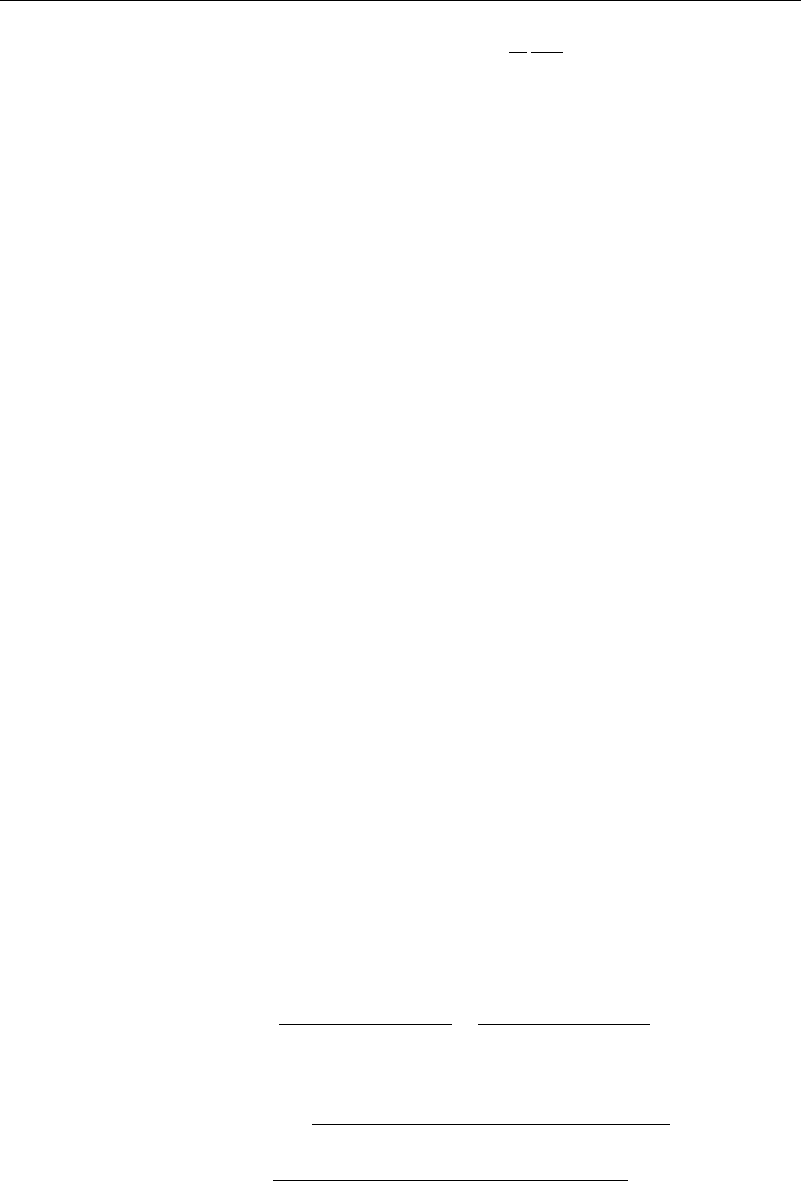
Figure 12.2.1a Computational molecule for the relaxation method

–

–16

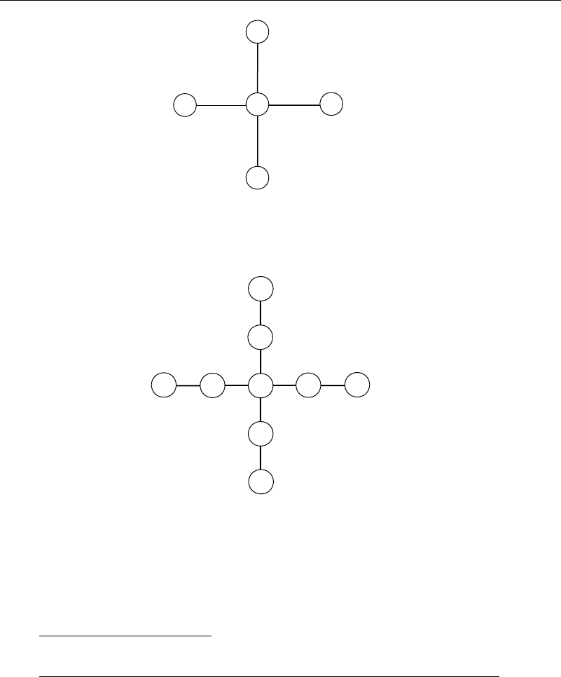
Figure 12.2.1b Computational molecule for the SOR method

to fourth-order accuracy. The computational molecules for the two cases are shown in

Figures 12.2.1a and b. When x = y, these equations reduce to

jk

≈

j+1k

j−1k

jk+1

jk−1

 (12.2.1a)

jk

≈



−V

j+2k

+16V

j+1k

+16V

j−1k

−V

j−2k





−V

jk+2

+16V

jk+1

+16V

jk−1

−V

jk−2





(12.2.2a)

If the values of the function V are known on the boundary (Dirichlet problem),

such as when posing a flow situation in terms of a stream function, the boundary con-

ditions are easily handled. If the normal derivatives of the function V are known on

the boundary (Neumann problem), such as when solving for the velocity potential,

the boundary conditions require additional equations to accommodate the derivatives.

In analyzing a given flow using the velocity potential, the body shape and the nor-

mal derivatives are known on the surface, so this is a Neumann problem and the

286 Multidimensional Computational Methods

pressure coefficient can be found. In the case of a design problem, the body shape is

unknown except for the fact that it is a stream surface, and dealing with it as a Dirich-

let problem has advantages. Often the pressure coefficient is also known in a design

situation.

The resulting algebraic equations can be handled in a number of ways.

1. Use traditional methods such as Gaussian elimination. Unfortunately this will

require N +1! multiplications (N being the number of nodes), and possible round-off

errors can be introduced in the solution process.

2. Use the relaxation method. For the case with Dirichlet conditions and a square

grid, for second-order accuracy use equation (12.2.1a) in the form

i+1

jk

≈

j+1k

j−1k

jk+1

jk−1

 (12.2.1b)

The superscript denotes the number of the sweep through all of the nodes. Start off

by assigning arbitrary values to all nodes. This is sweep number 0. Use your best

judgement in assigning these first values, but it is not necessary to be perfectly accu-

rate. Next, go from point to point, changing the value of the point you are at to

the average of its neighbors (sweep number 2). After you have swept through every

point, repeat the process again and again until the change is negligible. In prac-

tice, rather than using old values of V in computing the right-hand side of equation

(12.2.1b), the most recently computed values are used, thus speeding up the process

slightly.

While such a boring procedure is perfectly designed for a computer, it is sobering

to reflect that in days gone by this was done with an adding machine (or maybe not),

pencil, paper, eraser, and a human!

3. Use the successive over-relaxation method (SOR). In this case equation (12.2.1a)

is replaced by

i+1

jk

≈V

jk





j+1k

j−1k

jk+1

jk−1

−4V

jk



 (12.2.1c)

Again, the i superscript denotes the number of the integration, and  is a parameter

between 1 and 2 used to speed up the calculations. The “best” value of  to use for a

particular problem is determined by making a few trial runs for various values of ,

which can be time-consuming. Choosing a value somewhere around 1.7 or so does a

good job.

4. Use the successive line over-relaxation method (SLOR). This is the same

as the SOR method, but rather than going around from point to point, a row

of points (line) is solved using previous values and a method such as Gauss

elimination.

5. If information is sought only in a particular region, random walk techniques can

be useful. If you want to find the value at a point j k, for example, start at that point

and randomly choose one of the numbers 1 to 4 (1 to 6 for three-dimensional problems).

Do this until a boundary point is reached, where the value of V is B

, the i standing for

the ith iteration. Repeat this process N times. Then V

jk

≈



i=1

, where N

is the

12.2 Relaxation Methods 287

number of steps needed to get to the boundary point with value B

and N



i=1

is the total number of steps. The accuracy increases as N

−4

, but clearly many, many

steps must be taken.

6. Write the N algebraic equations in N unknowns, and use a traditional algebraic

solver. The algebraic equations are sparse, which helps, but the fact that the matrix

of the coefficients is not narrow-banded means that special methods tailored to such a

problem must be used. These and other procedures can be found in much more detail

in Smith (1978), for example.

In the preceding, attention has been paid only to the case where boundaries are

rectangular, a fairly restricted case. For irregular boundaries, one could rephrase equation

(12.2.1) in a mesh of unequal sides, but then a good part of the computational problem

is to determine which boundary point you are near and which variation of equation

(12.2.1) is needed. Also, near corners, where changes in the solution can be rapid,

accuracy can be lost unless the grid mesh is shrunk. Two (at least) methods have been

introduced to overcome this problem.

The ideas of conformal mapping introduced in Chapter 3 are ideally suited to

generate grids to fit boundaries of any shape. Thomson, Warsi, and Mastin (1985)

present techniques useful in both two and three dimensions for computer generation

of grids for all three classes of partial differential equations. Basically, they use the

conformality of analytic functions to map the flow space into a rectangle. Control

functions can be used to adapt the grid spacing so that spacing is small and cell count

denser where the gradient of the function can be expected to be large. After the space is

transformed to the rectangle, the equations of interest are also transformed to the new

coordinate system and then solved.

The finite element method (FEM, also sometimes FEA for finite element analysis),

introduced for one-dimensional problems in Chapter 11, can also be adapted to two- and

three-dimensional problems. Programs usually come as a package, including grid gener-

ation and solvers. Grid generation is to some degree usually automatic, with provisions

for intervention by the user where refinements in the grid are needed. Elements used

can be rectangular, triangular, semi-infinite, and a variety of others. The polynomials

used on the sides of the elements vary in complexity, depending on the accuracy and

order of the derivatives needed.

FEM was originally developed for solution of problems in the linear theory of elas-

ticity, where the equations are strongly elliptic. In elasticity theory energy is conserved,

and only the “laminar” state exists. Thus, one would expect that, unless special provi-

sions are made for fluid flow problems, there would be a Reynolds number limitation

on computational accuracy. Upwind differencing, described later, has made it possible

to extend this limitation somewhat, and great claims have been made for the commer-

cial programs. Many even claim to handle turbulent flows. However, since many of

the companies are secretive as to how Reynolds number limitations and turbulence are

treated, it is difficult to assess their claims.

FEM programs can be used for irrotational flows with cavities. A simple approach

is to first estimate the shape of the cavity, then correct the shape to make it tangent

to the computed velocity. In the process, all nodes on the cavity are moved by the

process. It is to be repeated until some error norm such as



all cavity nodes

y

new

−y

old



is less than some value. Other methods for cavity flows have been suggested (e.g.,

Brennen, 1969).

288 Multidimensional Computational Methods

12.3 Surface Singularities

To illustrate the use of surface singularities in two-dimensional flows, the basic starting

point is Cauchy’s integral formula, which states that for any analytic function (i.e., one

that satisfies the Cauchy-Riemann conditions)

fz =

2i



f

 −z

d (12.3.1)

where the integration is about a closed path traversed in the positive sense. That is, as

the path of integration is traversed, the direction taken is such that the interior is always

to the left. If z is within the closed path, the integral is zero.

Since the complex velocity

is an analytic function, we can write

u −iv =

2i



u −iv

 −z

d (12.3.2)

Letting d =e

i

ds, where ds is real and  represents the slope of the integration path,

equation (12.3.2) becomes



u −iv



d =



u −iv



i

ds =



tangent

−iq

normal



ds

where q

tangent

and q

normal

are the tangent and normal velocity components with respect

to the path. Thus, equation (12.3.2) becomes

u −iv =

2i



tangent

−iq

normal

 −z

ds =



normal

2

z −



tangent

2

z −

 (12.3.3)

Recalling that

u −iv

source

2

z −

and u −iv

vortex

i

2

z −



it is seen that the first integral represents a source distribution, while the second integral

can be interpreted as a vortex distribution. Notice as shown in Chapter 2, that a vortex

distribution and a doublet distribution are equivalent.

In Chapter 2 the panel method was discussed for finding the flow about a submerged

body. We next show how for two-dimensional inviscid flows this can be implemented

numerically for lifting bodies.

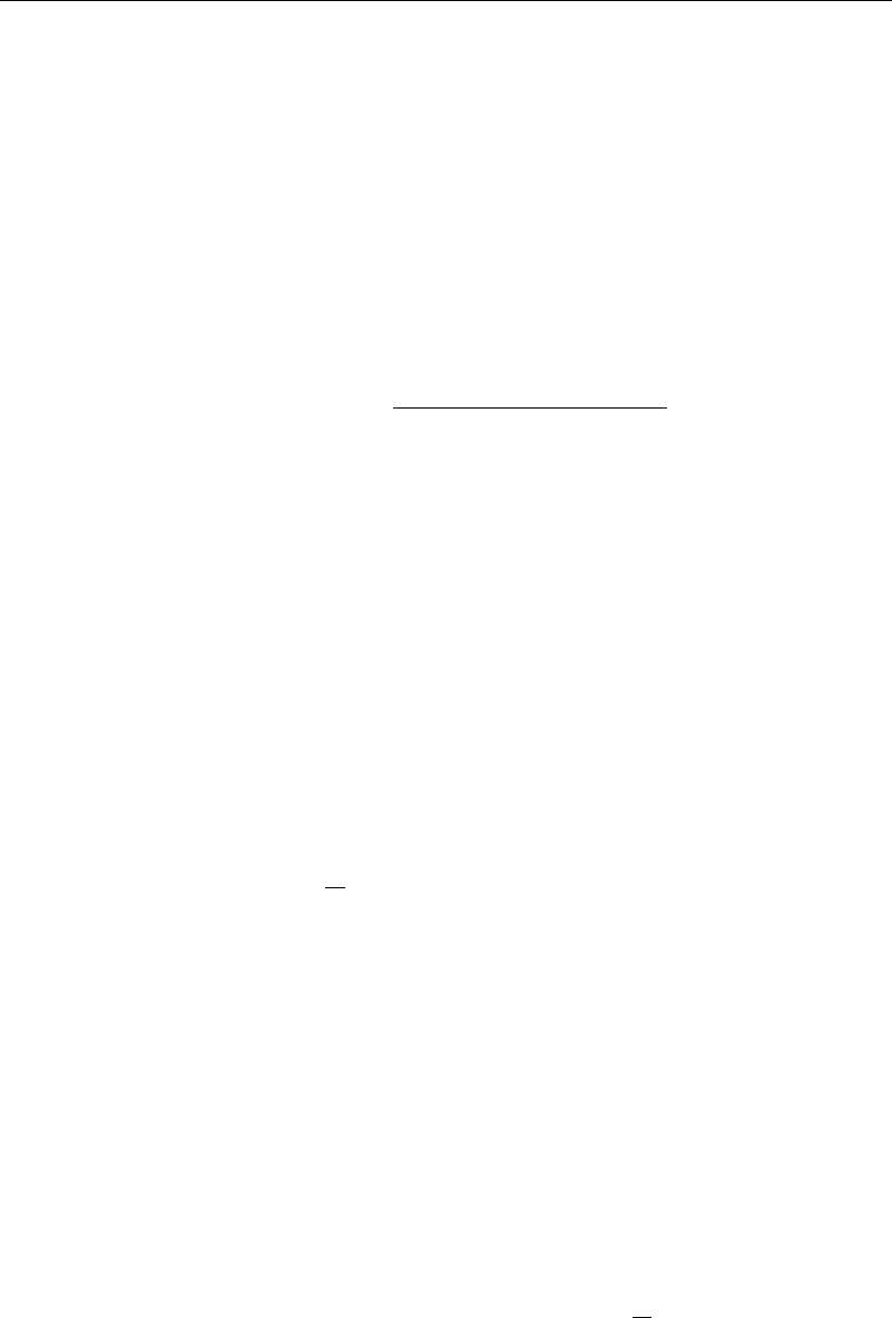
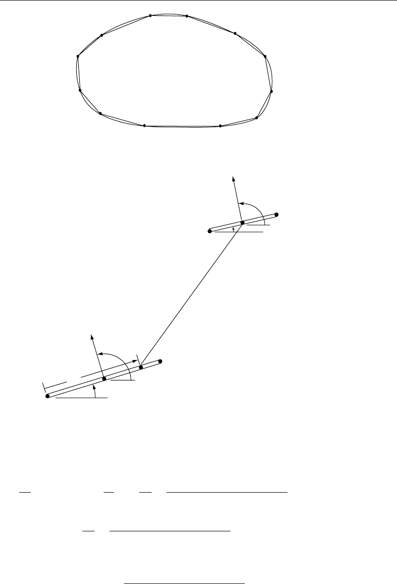
First, consider a closed two-dimensional body made up of a series of N flat panels.

An example is shown in Figure 12.3.1, where 12 panels are inscribed within the body.

Each panel has a source and a vortex on it. The strength of each source and vortex is

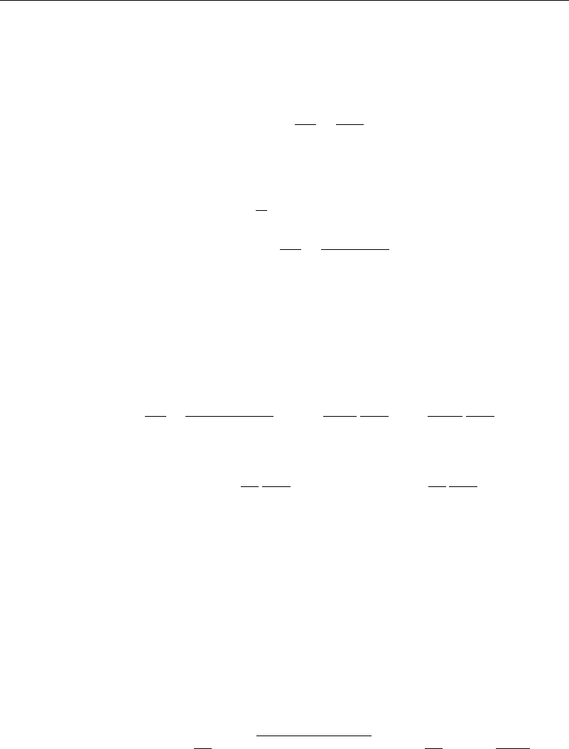
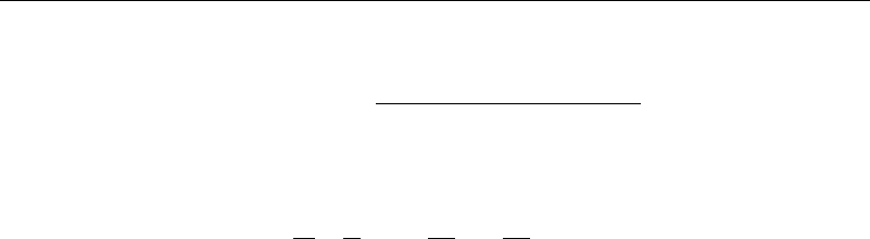
constant on a panel but can differ from panel to panel. Two such panels are shown in

Figure 12.3.2 to illustrate the geometry. The velocity potential then contains the uniform

stream plus the contributions from each of the N panels—that is,

x y = Ux +



j=1

2





x −x





+y −y







j=1



2



tan

−1

y −y



x −x





(12.3.4)

The control points where the boundary will be taken are at the center of each panel and

designated by x

y

. (Note: Panels can be constructed so either their endpoints lie on

the surface of the body or the control points lie on the body. Some evidence suggests

that the latter is more accurate.)

12.3 Surface Singularities 289

P10

P11

P12

Figure 12.3.1 Panel method—numbering of panels

i th panel

panel

i + 1

, Y

i + 1

)

j + 1

, Y

j + 1

)

, y

)

, Y

)

, y

)

, Y

)

, y

)

∼∼

Figure 12.3.2 Panel method—definitions

Applying the boundary conditions, find that



n



y

=U cos



j=1

j=i

2



x −x



 cos 

+y −y



 sin 

x −x





+y −y







j=1



2



x −x



 sin 

−y −y



 cos 

x −x





+y −y







(12.3.5)

Let



x −x



 cos 

+y −y



 sin 

x −x





+y −y





(12.3.6)

290 Multidimensional Computational Methods

for the sources and





x −x



 sin 

−y −y



 cos 

x −x





+y −y





(12.3.7)

for the vortices. Then





j=1

j=i



2



2





=−U cos 

 (12.3.8)

The first thing to notice is that by applying the boundary conditions, there are N

equations in 2 N unknowns. The Kutta condition also has not yet been applied, which

is necessary for a lifting body. Notice also that in using either source or vortex panels,

the tangency condition is satisfied only at the control points, and the velocity is infinite

at every panel edge.

There are a number of approaches that can be used to model a lifting surface and

balance the number of equations and unknowns in the process.

1. Use a unique source strength and the same vortex strength on every panel,

giving N +1 unknowns. Impose the tangency condition at N control points, and

also impose one Kutta condition at the trailing edge. This a fully determinate

system.

2. Use a unique source and a parabolic vorticity distribution on the top and bottom

panels. Let top and bottom maximum vortex strengths have the same magnitude

so that there are N +1 unknowns. Tangency conditions at N control points and

one Kutta condition make this a fully determinate system.

3. Use a unique source and vortex strength on each panel, giving 2N unknowns. Use

two control points on each panel and one Kutta condition. This an indeterminate

system, requiring a least squares procedure or something similar to resolve the

inconsistency.

4. Use a unique source and vortex on each panel, giving 2N unknowns. Use two

control points on each panel and one Kutta condition. This an indeterminate

system, requiring a least squares procedure or something similar.

5. Use a unique source and the same vorticity on each panel, giving N +1

unknowns. Use two control points on each panel and one Kutta condition.

This an indeterminate system, requiring a least squares procedure or a similar

technique.

6. Use a unique vortex on each panel, giving N unknowns. Satisfy tangency at

one control point on each panel and one Kutta condition. This an indeterminate

system, requiring a least squares procedure or something similar.

7. Use a unique vortex on each panel, giving N unknowns. Use two control points

on each panel and one Kutta condition. This an indeterminate system, requiring

a least squares procedure or something similar.

8. Use curved panels, perhaps parabolic or cubic in shape, along with singularity

distributions that vary on each panel. This would be particularly advantageous

12.3 Surface Singularities 291

near the rounded nose of an airfoil, where otherwise the number of panels

must be increased to fit the geometry. The number of variations on this is

unlimited.

Indeterminate systems can be handled as follows:

If the given system is



j=1

i=1 2NN+1N+M, let

N +M



i=1





j=1

−b



 (12.3.9)

Then, to minimize E

, let

E

x

N +M



i=1





j=1

−b



=0 (12.3.10)

Then



j=1



N +M



i=1



N +M



i=1

k=1 2N (12.3.11)

This system is determinate.

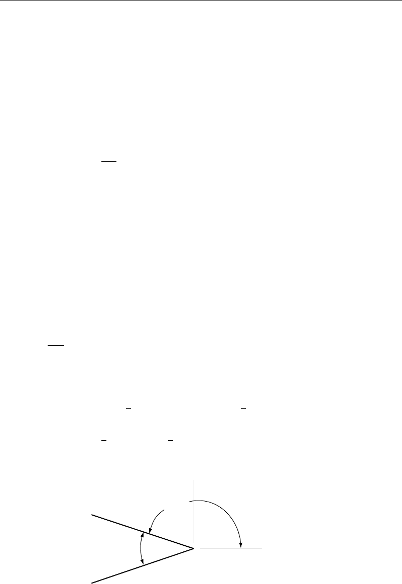
There are several approaches possible for satisfying the Kutta condition. For

example, if a body shape with a sharp trailing edge is to be modeled, the Kutta

condition could be imposed at the trailing edge. Consider the two panels surround-

ing the trailing edge, as shown in Figure 12.3.3. Locally the complex potential will

look like

w = Az

n−1

 (12.3.12)

where n =

2

2−

and  is the wedge angle. Denoting the tangent velocities on the top

panel (panel #1, length S

) and the bottom panel (panel #N, length S

), the Kutta

condition requires that the velocities be the same on these two panels. The velocities at

the control points are

=nA





n−1

v

=−nA





n−1



therefore v





1−n





1−n

=0

(12.3.13)

π – κ /2

Figure 12.3.3 Kutta condition—first method

292 Multidimensional Computational Methods

CP3

CP2

CP1

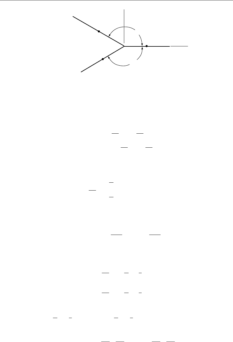
Figure 12.3.4 Kutta condition—second method

An alternate way of meeting the Kutta condition is shown in Figure 12.3.4. Here

an extra panel of length S

has been added at the trailing edge. Take the lengths of the

three panels be given as s

s

. The result is then

wz =

⎧

⎪

⎨

⎪

⎩

/

=Ar

/



cos





+i sin







 0 ≤ ≤ 

/−1

=Br

/−1



cos





+i sin







 − ≤  ≤0

(12.3.14)

giving

⎧

⎪

⎨

⎪

⎩





/−1

 0 ≤ ≤ 





/−2

 − ≤  ≤0

(12.3.15)

Then at control point 3 there is a discontinuity in  of magnitude

 =A



2s



/

−B



2s



/

 (12.3.16)

The velocities at control points 1 and 2 are



cp1







s



/−1

and



cp2







s



/−1



(12.3.17)

Thus A =







s



1−/

B=







s



1−/

,so

 =V

s



s



/

+V

s



s



/

 (12.3.18)

12.3 Surface Singularities 293

It is next necessary to carry out the integrations and put our equations in final form.

With the help of Figure 12.3.2, letting ˜x

cos

 ˜y

sin 

, then

=X

−x

 cos 

+Y

−y

 sin 



=X

−x



+Y

−y



 (12.3.19)

=−X

−x

 sin 

+Y

−y

 cos 



and

sin

−

 ln



S

+2A





−cos

−





tan

−1

−tan

−1





(12.3.20)

Similarly



=−

cos

−

 ln



S

+2A





−sin

−





tan

−1

−tan

−1





(12.3.21)

With these at hand, a choice can be made as to the number of sources and vortices to

retain.

Note that from the point of view of the calculations, just having a determinate system

may not be sufficient for obtaining good results. Some of the combinations of sources

and vortices result in stiff systems. This means that when a system of equations such

as (in matrix form) Ax =B is being solved, such a system has a set of eigenfunctions

and eigenvalues given by Ay

= 

. If the eigenvalues are all of the same order of

magnitude, the problem is not stiff, and the equation can be solved by standard methods.

If, however, there is a large disparity in the magnitude of the eigenvalues, then the

problem is stiff and is said to be ill-conditioned—that is, it is very sensitive to small

changes in the magnitudes of terms in either the matrix A or the known vector B.

Generally, it is not practical to first compute all of the eigenvalues to see whether

the system is stiff. It is better to solve the problem and then use back substitution or

some other check to see whether the solution is accurate. If it turns out that the method

you selected results in a stiff system, there are specialized methods that are designed

for dealing with stiff systems. It may, however, be much easier to select a different

combination of sources and vortices.

Notice that having a wide range in magnitude of the eigenvalues is reminiscent of

the boundary layer, where there are large gradients within the boundary layer and much

smaller ones outside it. It should come as no surprise that stiffness questions arise there

as well.

Here are some tips for maintaining accuracy. Rubbert and Saaris (1972) recommend

using double sheets of vortices inside the body. The following should be observed:

1. It is not necessary to place singularities on the boundary; they may be placed

within the boundary. If a single vortex is inserted in a thin body, the sources

above and below the vortex, the sources tend to be of opposite signs and act

like a doublet, with the strength inversely proportional to the distance between

them. This gives a strong gradient in source strength, which is to be avoided.

2. A series of vortices that are inserted with a strength approximating the load

distribution generally gives good results. However, if the angle of attack is to be