Gibilisco S. Everyday Math Demystified: A Self-Teaching Guide

Подождите немного. Документ загружается.

2 3 2 SUBSTITUTION METHOD

Consider a 2  2 set of linear equations in the above form. The substitution

method of solving these equations consists in performing either of the follow-

ing sequences of steps. If a

6¼ 0, use Sequence A. If a

¼ 0, use Sequence B.

If both a

¼ 0 and a

¼ 0, the set of equations is in fact a pair of equations

in terms of a single variable, and the following steps are irrelevant.

Sequence A. First, solve the ﬁrst equation for x in terms of y:

x þ b

y þ c

¼ 0

x ¼b

y  c

x ¼ðb

y  c

Þ=a

Next, substitute the above-derived solution for x in place of x in the second

equation from the original pair, obtaining:

½ðb

y  c

Þ=a

þb

y þ c

¼ 0

Solve this single-variable equation for y, using the previously outlined rules

for solving single-variable equations. Assuming a solution exists, it can be

substituted for y in either of the original equations, deriving a single-variable

equation in terms of x. Solve for x, using the previously outlined rules for

solving single-variable equations.

Sequence B. Because a

¼ 0, the ﬁrst equation has only one variable, and is

in the following form:

y þ c

¼ 0

Solve this equation for y:

y ¼c

This can be substituted for y in the second equation from the original pair,

obtaining:

x þ b

ðc

Þþc

¼ 0

x  b

ðc

Þþc

¼ 0

x ¼ b

ðc

Þc

x ¼½b

ðc

Þc

=a

CHAPTER 5 Basic Algebra 111

2 3 2 ADDITION METHOD

Consider again the following set of two linear equations in two variables:

x þ b

y þ c

¼ 0

x þ b

y þ c

¼ 0

where a

, a

, b

, c

, and c

are constants, and the variables are represented

by x and y. The addition method involves performing two separate and

independent steps:

Multiply one or both equations through by constant values to cancel

out the coeﬃcients of x, and then solve for y.

Multiply one or both equations through by constant values to cancel

out the coeﬃcients of y, and then solve for x.

The scheme for solving for y begins by multiplying the ﬁrst equation through

by  a

, and the second equation through by a

, and then adding the two

resulting equations:

a

x  a

y  a

¼ 0

x þ a

y þ a

¼ 0

ða

 a

Þy þ a

 a

¼ 0

Next, add a

to each side, obtaining:

ða

 a

Þy þ a

¼ a

Next, subtract a

from each side, obtaining:

ða

 a

Þy ¼ a

 a

Finally, divide through by a

 a

, obtaining:

y ¼ða

 a

Þ=ða

 a

For this to be valid, the denominator must be nonzero. This means the

products a

and a

must not be equal to each other.

The process of solving for x is similar. Consider again the original set of

simultaneous linear equations:

x þ b

y þ c

¼ 0

x þ b

y þ c

¼ 0

PART 2 Finding Unknowns

112

Multiply the ﬁrst equation through by  b

, and the second equation through

by b

, and then add the two resulting equations:

a

x  b

y  b

¼ 0

x þ b

y þ b

¼ 0

ða

 a

Þx þ b

 b

¼ 0

Next, add b

to each side, obtaining:

ða

 a

Þx þ b

¼ b

Next, subtract b

from each side, obtaining:

ða

 a

Þx ¼ b

 b

Finally, divide through by a

 a

, obtaining:

x ¼ðb

 b

Þ=ða

 a

For this to be valid, the denominator must be nonzero; this means

6¼ a

WHERE TWO LINES CROSS

When you have a pair of linear equations in two variables, you can graph

them both, and they will always both appear as straight lines. Try this

with several diﬀerent pairs of linear equations, letting the horizontal

axis show x values and the vertical axis show y values. Usually, the two

lines intersect at some point, although once in a while they are parallel,

and don’t intersect anywhere.

The solution to a pair of linear equations in two variables (if a solution

exists) corresponds to the x and y values of the intersection point for the

lines representing the equations. If the two lines are parallel, then there is

no solution.

Graphing a pair of linear equations is not a good way to ﬁnd the solution,

or even of determining whether or not a solution exists. This is because

graphing is a tedious and approximate business. It’s a lot of work to generate

the graphs for a pair of equations, and once you have drawn them, ﬁguring

out where (or even if) the lines intersect is subject to estimation errors. It’s

easiest to solve 2  2 sets of linear equations using the addition method.

That’s the scheme that we’ll use in the next two problems. We’ll graph them,

too, but only as an aid to visualizing the situations.

CHAPTER 5 Basic Algebra 113

PROBLEM 5-4

Use the 2  2 addition method to solve the following pair of linear equations,

reducing them to standard form and then ‘‘plugging in’’ the constants to the

general equations for x and y derived above.

2x  y ¼ 2

x þ 3y ¼3

SOLUTION 5-4

To convert the ﬁrst equation to standard form, subtract 2 from each side. To

convert the second equation to standard form, add 3 to each side. This gives

us the following:

2x  y  2 ¼ 0

x þ 3y þ 3 ¼ 0

The constants in the ﬁrst equation are a

¼ 2, b

¼1, and c

¼2. The con-

stants in the second equation are a

¼1, b

¼ 3, and c

¼ 3. Therefore, we

can solve for x by ‘‘plugging in’’ the appropriate constants to the following

general equation:

x ¼ðb

 b

Þ=ða

 a

¼½3 ð2Þð1Þ3=½ð1Þð1Þ2  3

¼½6 ð3Þ=ð1  6Þ

¼ð3Þ=ð5Þ

¼ 3=5

We can solve for y by ‘‘plugging in’’ the appropriate constants as follows:

y ¼ða

 a

Þ=ða

 a

¼ ½ð1Þð2Þ2  3=½2  3 ð1Þð1Þ

¼ð2  6Þ=ð6  1Þ

¼4=5

Thus, x ¼ 3/5 and y ¼4/5. Sometimes this is expressed by writing the

numbers one after the other, between parentheses, separated by a comma,

but without any space after the comma:

ðxóyÞ¼ð3=5ó  4=5Þ

PART 2 Finding Unknowns

114

PROBLEM 5-5

Use the 2  2 addition method to solve the original pair of equations from

the previous problem directly, rather than by substituting constants into

the general forms of the equations.

SOLUTION 5-5

Here are the original two equations again:

2x  y ¼ 2

x þ 3y ¼3

To solve for x, we must get the y terms to cancel out when we add the two

equations. This can be accomplished by multiplying both sides of the top

equation by 3 and then adding the two resulting equations together:

6x  3y ¼ 6

x þ 3y ¼3

5x ¼ 3

Then divide both sides of this equation by 5 to get x ¼ 3/5.

To solve for y, we must get the x terms to cancel out when we add the two

equations. In order to make this happen, multiply both sides of the bottom

equation by 2, and then add the two resulting equations together:

2x  y ¼ 2

2x þ 6y ¼6

5y ¼4

Then divide both sides by 5 to get y ¼4/5.

PROBLEM 5-6

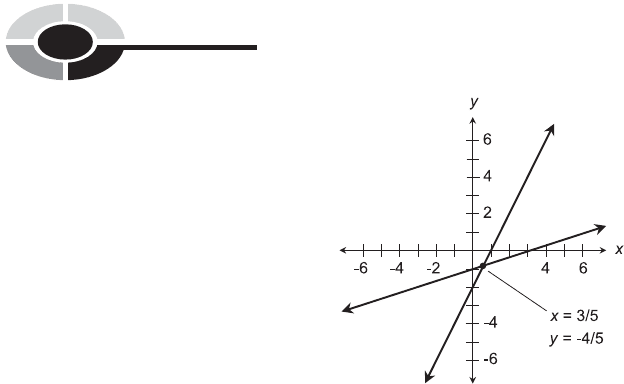
Draw the straight-line graphs from the two equations in Problems 5-4 and

5-5, showing their intersection point at (x,y) ¼ (3/5, 4/5).

SOLUTION 5-6

We haven’t learned the quick-and-easy way to graph linear equations yet.

That stuﬀ is reserved for a later chapter. For now, just pick some numbers

for x and plot the resulting points for y. Two points should do for both

equations, because we know they’ll be straight lines; from basic geometry

we know that any straight line can be uniquely determined by two points.

The result should look like Fig. 5-5.

CHAPTER 5 Basic Algebra 115

Quiz

Refer to the text in this chapter if necessary. A good score is eight correct.

Answers are in the back of the book.

1. Which of the following is not a legitimate way to manipulate an

equation in which the variable is x?

(a) Subtract 1 from both sides.

(b) Divide both sides by 0.

(d) Add 2x to both sides.

2. The term ‘‘linear,’’ when used to describe an equation, comes from

the fact that

(a) such equations look like straight lines when graphed in two

variables

(b) the variables change at constant rates

(d) the variables are actually constants

3. The solution to the equation 3x þ 7 ¼2x þ 3is

(a) undeﬁned

(b) equal to any and all real numbers

(d) equal to 5/4

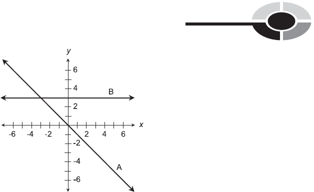
4. Suppose the two straight lines in Fig. 5-6 represent linear equations

in standard form, except that the 0 on the right-hand side of the

Fig. 5-5. Illustration for Problem 5-6.

PART 2 Finding Unknowns

116

equals sign is replaced by y. Examine line A. It appears from this

graph that when y ¼ 0, the value of x

(a) is equal to 0

(b) is positive (greater than 0)

(d) is not deﬁned

5. Suppose the two straight lines in Fig. 5-6 represent linear equations in

standard form, except that the 0 on the right-hand side of the equals

sign is replaced by y. Examine line A. It appears from this graph

that when y is positive (greater than 0), the value of x

(a) is equal to 0

(b) is positive (greater than 0)

(d) is not deﬁned

6. Suppose the two straight lines in Fig. 5-6 represent linear equations in

standard form, except that the 0 on the right-hand side of the equals

sign is replaced by y. Examine line B. It appears from this graph that

when y ¼ 0, the value of x

(a) can be any real number

(b) is positive (greater than 0)

(d) is not deﬁned

7. Suppose the two straight lines in Fig. 5-6 represent linear equations in

standard form, except that the 0 on the right-hand side of the equals

Fig. 5-6. Illustration for Quiz Questions 4 through 7.

CHAPTER 5 Basic Algebra 117

sign is replaced by y. Examine line B. It appears from this graph that

when y ¼ 3, the value of x

(a) can be any real number

(b) is positive (greater than 0)

(d) is not deﬁned

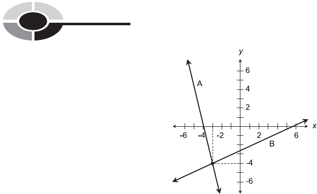
8. Examine Fig. 5-7. Suppose lines A and B represent a pair of linear

equations in two variables, x and y. How many solutions exist to

this pair of equations?

(a) None.

(b) One.

(d) Inﬁnitely many.

9. Which of the following statements is true of any or all solutions (x, y)

to the pair of linear equations shown by lines A and B in Fig. 5-7?

(a) x ¼3

(b) y ¼3

(d) x þ y ¼3

10. What is the unique solution (x, y) to the equation 2x þ 2y ¼ 0?

(a) x ¼2

(b) y ¼2

(d) An additional equation in x and y is necessary to answer this.

Fig. 5-7. Illustration for Quiz Questions 8 and 9.

PART 2 Finding Unknowns

118

CHAPTER

More Algebra

When the variable, or unknown, in an equation is raised to a power, things

get interesting. The larger the exponents attached to the variables, the more

interesting things become, and the more diﬃcult it gets to solve the equation.

In this chapter, we’ll look into the basics of quadratic, cubic, and higher-

order equations in one variable. Even if you’re not a mathematician or a

scientist, you’ll encounter equations like these once in a while, so it’s good

to know about them.

Quadratic Equations

A one-variable, second-order equation, also called a second-order equation in

one variable or, more often, a quadratic equation, can be written in the follow-

ing standard form:

þ bx þ c ¼ 0

where a, b, and c are constants, a is not equal to 0, and x is the variable.

The constants a, b, and c are also known as coeﬃcients.

119

SOME EXAMPLES

Any equation that can be converted into the above form is a quadratic

equation. Alternative forms are:

þ nx ¼ p

¼ rx þ s

ðx þ tÞðx þ uÞ¼0

where m, n, p, q, r, s, t, and u are constants. Here are some examples of

quadratic equations in various forms:

þ 2x þ 1 ¼ 0

3x

 4x ¼ 2

¼3x þ 5

ðx þ 4Þðx  5Þ¼0

GET IT INTO FORM

Some quadratic equations are easy to solve. Others are diﬃcult. The ﬁrst step

in ﬁnding the value(s) of the variable in a quadratic is to get the equation

either into standard form or into factored form.

The ﬁrst equation above is already in standard form. It is ready for an

attempt at solution, which, as we will shortly see, is easy.

The second equation above can be reduced to standard form by

subtracting 2 from each side:

3x

 4x ¼ 2

3x

 4x  2 ¼ 0

The third equation above can be reduced to standard form by adding 3 x to

each side and then subtracting 5 from each side:

¼3x þ 5

þ 3x ¼ 5

þ 3x  5 ¼ 0

An interesting aside: these are not the only ways the equations can be reduced

to standard form. They can be multiplied through by any nonzero constant,

and the resulting equations are still in standard form.

PART 2 Finding Unknowns

120