Gerya T. Introduction to Numerical Geodynamic Modelling
Подождите немного. Документ загружается.

Programming exercises and homework 217
approach allows us to reach computer accuracy solution within a finite amount
of iterations, even for very large viscosity contrasts (Fig. 14.13). An example
of using such algorithm (Fig.14.13) is given in the program Variable_viscosity_
MultiMultigrid_arbitrary.m.
Finally, it is also important to mention that besides large viscosity contrasts,
further convergence problems can be caused by strongly irregular grid spacing, by
significant differences in grid spacing used for different dimensions, by strong (e.g.
plastic) localisation of deformation characterising a mechanical solution at the finest
grid which is not captured on coarser levels etc. Therefore, be prepared that some
of your thermomechanical models which utilise multigrid will be ‘demanding’,
and will require special efforts in tuning and adjusting the iteration procedures.
Programming exercises and homework
Exercise 14.1
Program the multigrid solution based on a V-cycle for solving the Poisson equation
in 2D for the case of a circular planetary body embedded in a mass less-like
medium (Eqs. (14.6)–(14.16), Figs. 14.6–14.7). Use a ghost-node approach to
define the boundary conditions =0, along a circular boundary located at a
distance from the planet. Program a Poisson equation smoother based on Gauss–
Seidel iteration (Exercise 3.3 for Chapter 3) as an external MATLAB function and
call it for different levels of resolution. Program external functions for restriction
(Eq. (8.18), Fig. 8.8) and prolongation (Eq. (8.19), Fig. 8.9) operations to be
called for different multigrid levels. Model parameters: radius of the planet =
6000 km, density of the planet = 6000 kg/m
3
, model size = 18000 ×18000 km,
radius for gravity potential boundary = 8999 km, number of resolution levels =
4, resolution on the coarsest (last) grid = 7 ×7 nodal points, factor of increase in
resolution between the levels =2, relaxation coefficient for Gauss–Seidel iterations,
θ
Poisson
relaxation
= 1.5, number of smoothing iterations on the finest level = 5, factor of
increase in the number of iterations with the level coarsening =2. An example is in
Poisson_Multigrid_planet.m.
Exercise 14.2
Program a multigrid solution for solving the Stokes and continuity equations in 2D
for a constant viscosity case using a pressure–velocity formulation and a ghost-
node approach (Eqs. (14.20)–(14.44), Figs. 14.8–14.9). The setup corresponds to a
dense rectangular block sinking in the lower density medium. Model parameters:
model size = 100 ×100 km, block size =20 ×20 km (located in the middle of the
model), block density = 3100 kg/m
3
, medium density = 3000 kg/m
3
, acceleration
of gravity (vertical) =9.81 m/s
2
, model viscosity =10
20
Pa s, boundary conditions
218 The multigrid method
(a)
(b)
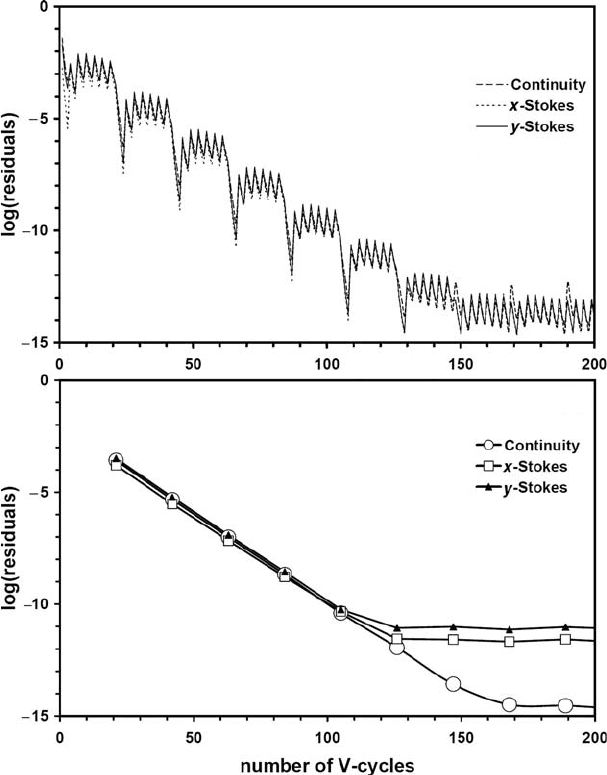
Fig. 14.13 Decay of normalised residuals for Stokes and continuity equations with
the number of multigrid V-cycles for a model with variable viscosity in the case
of a ‘multi-multigrid’ approach, which uses repetitive cycles of gradual increase
in computational viscosity contrast. Residuals stabilise at the computer accuracy
level. Five-level multigrid with resolution 49 ×49 points on the finest level are used
with relaxation parameters θ
continuity
relaxation
= 0.3 and θ
Stokes
relaxation
= 0.9. Numerical setup:
rectangular block having higher density and viscosity (by factor 10
6
) sinks into a
lower density and viscosity fluid. Iterations start from a hydrostatic pressure field
and zero velocities. (a) Decay of local residuals computed with current corrections
and right-hand side within each cycle (steps) of gradual viscosity contrast increase
(spikes). (b) Decay of global residuals computed after each cycle of gradual
viscosity contrast increase. Spikes in (a) are caused by an increase in viscosity
contrast by the factor of 10 every 3 multigrid cycles. Results are obtained with the
program Variable_viscosity_MultiMultigrid_arbitrary.m.
Programming exercises and homework 219
=free slip at all boundaries, number of resolution levels =4, resolution of the basic
grid on the coarsest (last) level =7 ×7 nodal points, factor of increase in resolution
between the levels =2, relaxation coefficients for Gauss–Seidel iterations, θ
Stokes
relaxation
=1.2 and θ
continuity
relaxation
=0.3, number of smoothing iterations on the finest (basic) level
= 5, factor of increase in the number of iterations with the level coarsening = 2.
An example is in Constant_Viscosity_Multigrid_ghost.m.
Exercise 14.3
Modify the previous example to include a variable viscosity (Eqs. (14.45)–
(14.55), Fig. 14.11). Use a high viscosity for the block (10
23
Pa s) in compar-
ison to the surrounding medium. Use θ
Stokes
relaxation
= 1.0 and θ
continuity
relaxation
= 0.3 and
program a gradual increase in the viscosity contrast by the factor of 10
1/2
(Eq.
(14.57)) to reach an accurate solution (Fig. 14.12). Example is in Variable_
viscosity_Multigrid_arbitrary.m.

15
Programming of 3D problems
Theory: Formulation of thermomechanical problems in 3D and its
numerical implementation. Numerical methods for solving temperature,
Poisson, momentum and continuity equations in 3D.
Exercises: Programming of numerical methods for temperature and
Poisson equations and coupled solving of momentum and continuity
equations in 3D.
15.1 Why simply not always 3D?
We know very well that the Earth is a 3D, nearly spherical object and, therefore, all
the dynamic processes inside our planet are inherently three dimensional. There-
fore, it is very logical to assume that realistic geodynamic modelling should always
be done in 3D. Also, if you talk to geoscientists studying various natural geological
objects, you are frequently told that such objects can only be modelled in 3D. This
is a normal expectation since they are perfectly aware of the spatial 2D variability
of geological structures on the Earth’s surface and they thus know that a similar
variability also exists in depth. Therefore, 3D modelling appears to be the natural
choice for ‘observers’. What about ‘modellers’? Why don’t they always use 3D
modelling? What’s wrong with it? The ‘uncensored’ truth about 3D modelling is
the following:
r
3D thermomechanical modelling is quite easy from a methodological point of view –
it is fairly straightforward to formulate and discretise the governing equations in a
3D Cartesian geometry for both simple viscous and more realistic visco-elasto-plastic
rheologies (especially by using the same relatively simple finite-differences and marker-
in-cell techniques that we extensively discussed in this book).
221
222 Programming of 3D problems
r
3D modelling is much more difficult from a technical point of view. This mainly concerns
the coupled solving of momentum and continuity equations. Highly accurate direct
solvers that are applicable in 2D are too slow and consume too much memory to yield
the same spatial resolution of numerical grids in 3D. Iterative solvers, on the other hand,
are very efficient for simple rheologies (such as constant viscosity problems) but do not
always converge well for realistic geodynamic problems, which involve large viscosity
contrasts on sharp interfaces.
It is obvious that when changing from 2D to 3D models, we do not want to
reduce the numerical resolution. This requirement, however, immediately implies
several orders of magnitude increase in the amount of grid points and markers and,
thus, in the amount of equations that have to be solved:
r
A 100 ×100 2D grid with 5 ×5 markers per cell implies around 3 ×100 ×100 =30 000
momentum and continuity equations to be solved and 5 ×5 ×100 ×100 = 250 000
markers to be followed at each time step;
r
A 100 ×100 ×100 3D grid with 5 ×5 ×5 markers per cell involves about 4 ×100 ×
100 ×100 = 4 000 000 momentum and continuity equations to be solved (i.e. 130 times
more than in 2D) and 5 ×5 ×5 ×100 ×100 ×100 =125 000 000 markers to be followed
at each time step (i.e. 500 times more than in 2D).
This is the reason why modellers prefer to apply 2D, rather then 3D approaches,
where geodynamic problems can be justifiably simplified to lower dimensions. 3D
geodynamic modelling is now developing very actively and significant progress is
already achieved in the field of mantle convection in both Cartesian and spheri-
cal geometry, in large-scale modelling of plate tectonics processes (especially in
modelling subduction) and in some other directions. Several groups are currently
working on the development of more efficient and universal all-in-one 3D numer-
ical geodynamic codes and 3D thermomechanical modelling is likely to become
a standard tool in all fields of computational geodynamics (see Kaus et al., 2008a
for an overview of the current state of the art).
This chapter gives a practical summary that allows a relatively simple implemen-
tation of 3D thermomechanical modelling, based on conservative finite-differences
and marker-in-cell techniques combined with iterative multigrid solvers similar to
those discussed in Chapter 14 for 2D problems.
15.2 3D staggered grid and discretisation of momentum, continuity,
temperature and Poisson equations
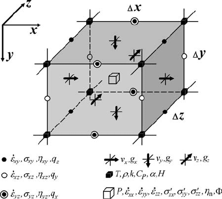
Let us first discuss the discretisation of various equations in 3D. Figure 15.1
shows an elementary volume (cell) of a 3D staggered grid that can be used for
discretisation of momentum, continuity, Poisson and temperature equations in the
case of viscous flow with variable viscosity and variable thermal conductivity. The
15.2 3D staggered grid, discretisation of equations 223
Fig. 15.1 Elementary volume (cell) of 3D staggered grid used for discretisation of
momentum, continuity, Poisson and temperature equations in the case of incom-
pressible viscous flow with variable viscosity and thermal conductivity.
grid is constructed in a specific way that allows a natural representation of all
governing equations with conservative finite differences:
r
pressure, deviatoric normal stresses and strain rates and gravity potential (when needed)
are located at the centre of the cell,
r
components of velocity vector v
x
, v
y
and v
z
and variable gravitational acceleration vector
g
x
, g
y
and g
z
(when needed) are located in the middle of the faces orthogonal to x, y and
z axes, respectively,
r
shear stresses and strain rates are located in the middle of the edges formed by the
intersection of faces containing respective velocity components, i.e. by intersection of
v
x
- and v
y
-faces in case of σ
xy
and ˙ε
xy
etc.,
r
viscosity is defined in four different places corresponding to positions of normal (η
n
,in
the centre of the cell) and shear (η
xy
, η
xz
, η
yz
, in the middle of respective edges) stress
components,
r
heat fluxes q
x
, q
y
and q
z
are located in the middle of edges parallel to x, y and z axes,
respectively,
r
other material properties and temperature are located at the cell corners, which are the
basic nodes of the grid.
Before discretising the governing equations on a 3D staggered grid, an important step
is (although it might sound really boring . . . ) to properly understand the indexing of
different field variables located around a grid cell (Fig. 15.1):
r
Indexing of variables located in the basic nodes (T, ρ, α, C
P
, etc.) of the grid is simple
since the respective arrays have dimension of N
x
×N
y
×N
z
, where N
x
, N
y
and N
z
are the
number of nodes of the basic grid in the respective directions.

224 Programming of 3D problems
(a)
(b)
(c)
Fig. 15.2 Distribution of various velocity nodal points in 3D in the case when
external nodes (open circles) are used to formulate boundary conditions for v
x
(a),
v
y
(b) and v
z
(c) velocity components. The basic grid of the model (see solid lines
in Fig. 15.1) is shown in grey.
r
Arrays for the variables located in cell centres (P, σ
xx
,η
n
, , etc.) will be (N
x
−1) ×
(N
y
−1) ×(N
z
−1).
r
Arrays for various shear stresses, strain rates and respective viscosity values located on
cell edges will be N
x
×N
y
×(N
z
−1) for σ
xy
,˙ε
xy
and η
xy
, N
x
×(N
y
−1) ×N
z
for σ
xz
,˙ε
xz
and η
xz
,(N
x
−1) ×N
y
×N
z
for σ
yz
,˙ε
yz
and η
yz
.
r
Finally, the indexing of the velocity nodes should take into account nodes located outside
the basic grid, which are used for formulating boundary conditions and interpolation
of velocity components to markers (similarly to ones that we discussed in Chapter 14
for 2D grids, Fig. 14.8). Consequently, velocity arrays will be larger in two direc-
tions compared to the basic grid resolution (Fig. 15.2): N
x
×(N
y
+1) ×(N
z
+1) for v
x
,
(N
x
+1) ×N
y
×(N
z
+1) for v
y
and (N
x
+1) ×(N
y
+1) ×N
z
for v
z
.
Based on these considerations, we can now understand the logic of indexing for
various grid points (Fig. 15.3) which will be then used to construct conservative 3D
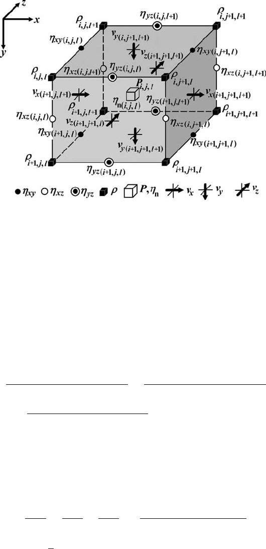
15.2 3D staggered grid, discretisation of equations 225
Fig. 15.3 Indexing of different variables for a 3D staggered grid (Fig. 15.1) with
external velocity nodes (Fig. 15.2).
finite-difference schemes for the momentum, continuity, Poisson and temperature
equations.
After extensive discussions on composing conservative FD schemes in 1D and
2D, the discretisation of various equations on a 3D staggered grid shown in
Figs. 15.1–15.3 is quite straightforward and therefore we only discuss it
briefly.
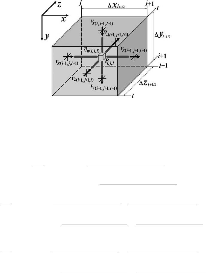
The representation of the incompressible 3D continuity equation on a stencil
with six velocity nodes around a cell (Fig. 15.4)is
v
x(i+1,j +1,l+1)
− v
x(i+1,j,l+1)
x
j+1/2
+
v
y(i+1,j +1,l+1)
− v
y(i,j+1,l+1)
y
i+1/2
+
v
z(i+1,j +1,l+1)
− v
z(i+1,j +1,l)
z
l+1/2
= 0, (15.1)
where i, j and l are indices in respectively y, x and z directions.
Discretisation of the Stokes equation for an incompressible fluid with variable
viscosity uses a stencil containing 15 velocity nodes and 2 pressure nodes. An
example of this stencil is shown in Fig. 15.5 for the case of the x-Stokes equation
∂σ
xx
∂x
+
∂σ
xy
∂y
+
∂σ
xz
∂z
− 2
P
i−1,j,l−1
− P
i−1,j −1,l−1
x
j−1/2
+ x
j+1/2
=
1
4
(ρ
i−1,j,l−1
+ ρ
i,j,l−1
+ ρ
i−1,j,l
+ ρ
i,j,l
)g
x
, (15.2)
226 Programming of 3D problems
Fig. 15.4 Stencil of a 3D staggered grid used for the discretisation of the continuity
equation for iterative solution. The small open cube in the centre corresponds to the
pressure node at which the continuity equation is formulated. Notation of different
nodal points is as in Fig. 15.1. Indexing of different variables corresponds to 3D
staggered grid with external velocity nodes (Fig. 15.3).
∂σ
xx
∂x
= 4η
n(i−1,j,l−1)
v
x(i,j+1,l)
− v
x(i,j,l)
x
j+1/2
(x
j−1/2
+ x
j+1/2
)
−4η
n(i−1,j −1,l−1)
v
x(i,j,l)
− v
x(i,j−1,l)
x
j−1/2
(x
j−1/2
+ x
j+1/2
)
, (15.3)
∂σ
xy
∂y
= 2η
xy(i,j,l−1)
v
x(i+1,j,l)
− v
x(i,j,l)
y
i−1/2
(y
i−1/2
+ y
i+1/2
)
+
v
y(i,j+1,l)
− v
y(i,j,l)
y
i−1/2
(x
j−1/2
+ x
j+1/2
)
−2η
xy(i−1,j,l−1)
v
x(i,j,l)
− v
x(i−1,j,l)
y
i−1/2
(y
i−3/2
+y
i−1/2
)
+
v
y(i−1,j +1,l)
− v
y(i−1,j,l)
y
i−1/2
(x
j−1/2
+x
j+1/2
)
,
(15.4)
∂σ
xz
∂z
= 2η
xz(i−1,j,l)
v
x(i,j,l+1)
− v
x(i,j,l)
z
l−1/2
(z
l−1/2
+ z
l+1/2
)
+
v
z(i,j+1,l)
− v
z(i,j,l)
z
l−1/2
(x
j−1/2
+ x
j+1/2
)
−2η
xz(i−1,j,l−1)
v
x(i,j,l)
− v
x(i,j,l−1)
z
l−1/2
(z
l−3/2
+ z
l−1/2
)
+
v
z(i,j+1,l−1)
− v
z(i,j,l−1)
z
l−1/2
(x
j−1/2
+ x
j+1/2
)
.
(15.5)
Discretisation of the y-Stokes and z-Stokes is rather obvious and the respective
conservative FD schemes can be constructed and indexed by analogy to Fig. 15.5
and Eqns. (15.2)–(15.5) (derive as an exercise).