Geiser J. Decomposition Methods for Differential Equations: Theory and Applications

Подождите немного. Документ загружается.

Numerical Experiments 127

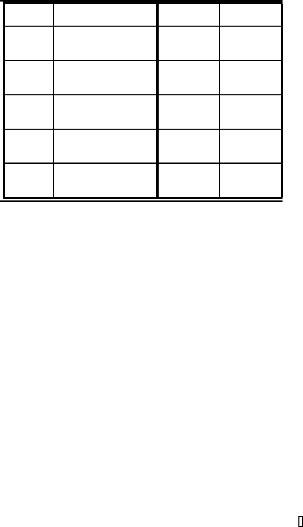
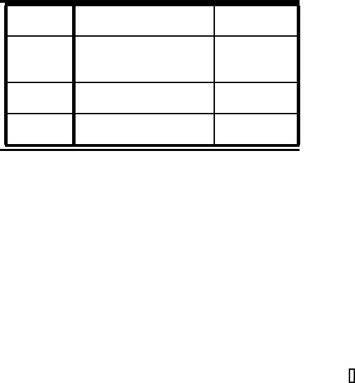
TABLE 6.5: Numerical results for the second example

with iterative splitting method and BDF3 method.

Iteration Number of err

err

steps i splitting partitions n

2 1 4.5321e-002 4.5321e-002

2 10 3.9664e-003 3.9664e-003

2 100 3.9204e-004 3.9204e-004

3 1 7.6766e-003 7.6766e-003

3 10 6.6385e-005 6.6385e-005

3 100 6.5312e-007 6.5312e-007

4 1 4.6126e-004 4.6126e-004

4 10 4.1334e-007 4.1334e-007

4 100 1.7864e-009 1.7863e-009

5 1 4.6833e-005 4.6833e-005

5 10 4.0122e-009 4.0122e-009

5 100 1.3737e-009 1.3737e-009

6 1 1.9040e-006 1.9040e-006

6 10 1.4350e-010 1.4336e-010

6 100 1.3742e-009 1.3741e-014

A higher order in the time discretization allows improved results with more

iteration steps. Based on the theoretical results, we can improve the order of

the results with each iteration step. Thus, for the fourth-order time discretiza-

tion, we can show the highest order in our iterative method. In comparison to

the nonsplitting method, with only applying the time discretization methods,

we can reach the same accuracy, but we have to take into account the in-

creased amount of computational time. An optimal choice of fewer iterations

and suﬃcient time partitions can save the resources, and we can propose it as

a competitive method.

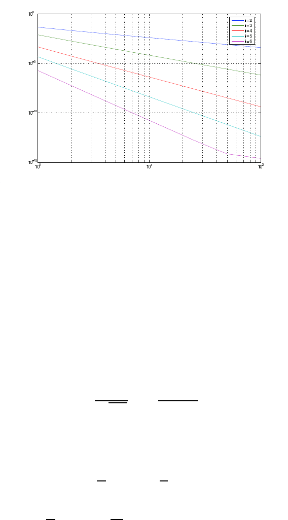
The convergence results of the three methods are given in Figure 6.1.

REMARK 6.2 For the nonstiﬀ case, we obtain improved results for

the iterative splitting method by increasing the number of iteration steps. Due

to improved time discretization methods, the splitting error can be reduced

with higher-order Runge-Kutta methods. Further, the optimal choice of it-

erations and suﬃcient time partitions can make the splitting method more

attractive to such standard problems. By the way, the application of such it-

erative splitting methods becomes more attractive for complicated equations,

while saving memory and computational time for the appropriate decomposi-

tion.

128Decomposition Methods for Diﬀerential Equations Theory and Applications

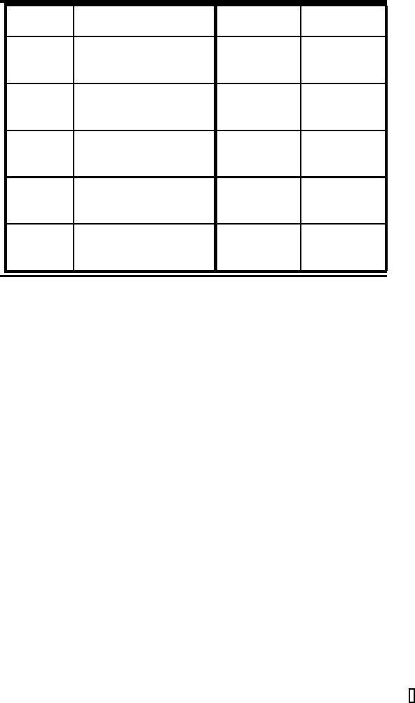
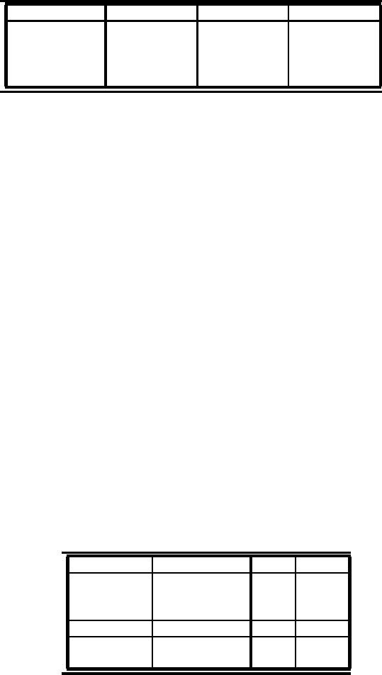
TABLE 6.6: Numerical results for the second example

with iterative splitting method and fourth-order Gauß-RK

method.

Iteration Number of err

err

steps i splitting partitions n

2 1 4.5321e-002 4.5321e-002

2 10 3.9664e-003 3.9664e-003

2 100 3.9204e-004 3.9204e-004

3 1 7.6766e-003 7.6766e-003

3 10 6.6385e-005 6.6385e-005

3 100 6.5369e-007 6.5369e-007

4 1 4.6126e-004 4.6126e-004

4 10 4.1321e-007 4.1321e-007

4 100 4.0839e-010 4.0839e-010

5 1 4.6833e-005 4.6833e-005

5 10 4.1382e-009 4.1382e-009

5 100 4.0878e-013 4.0856e-013

6 1 1.9040e-006 1.9040e-006

6 10 1.7200e-011 1.7200e-011

6 100 2.4425e-015 1.1102e-016

6.2.2.2 Linear ODE with Stiﬀ Parameters

We deal with the same equation as in the ﬁrst example, now choosing λ

and λ

=10

on the interval [0,1].

We therefore have the following operators:

A =



−10



,B=



010

0 −10



. (6.14)

The discretization of the linear ordinary diﬀerential equation is done with the

BDF3 method. Our numerical results are presented in Table 6.7. For the stiﬀ

problem, we choose more iteration steps and time partitions and show the

error between the analytical and numerical solution in the supremum norm

that is, err

= |u

k,exact

− u

k,num

| with k =1, 2.

In Table 6.7, we see that we must double the number of iteration steps to

obtain the same results for the nonstiﬀ case.

REMARK 6.3 For the stiﬀ case, we obtain improved results with

more than ﬁve iteration steps. Because of the inexact starting function, the

accuracy must be improved by more iteration steps. Higher-order time dis-

cretization methods, such as BDF3 method and iterative operator-splitting

method, accelerate the solving process.

Numerical Experiments 129

FIGURE 6.1: Convergence rates from two up to six iterations.

6.2.3 Third Example: Linear Partial Diﬀerential Equation

We consider the one-dimensional convection-diﬀusion-reaction equation given

R∂

u + v∂

u − D∂

u = −λu , in Ω × [t

end

), (6.15)

u(x, t

)=u

exact

(x, t

) , in Ω, (6.16)

u(0,t)=u

exact

(0,t) ,u(L, t)=u

exact

(L, t). (6.17)

We choose x ∈ [0,L]=ΩwithL =30andt ∈ [t

end

]=[10

, 2 · 10

Furthermore, we have λ =10

−5

, v =0.001, D =0.0001, and R =1.0. The

analytical solution is given by

exact

(x, t)=

√

Dπt

exp(−

(x − vt)

4Dt

)exp(−λt). (6.18)

To begin away from the singular point of the exact solution, we start from

thetimepointt

=10

Our split operators are

A =

∂

,B= −

(λ + v∂

). (6.19)

For the spatial discretization we use the ﬁnite diﬀerences with a spatial grid

width of Δx =

and Δx =

100

. The discretization of the linear ordinary

diﬀerential equation is accomplished with the BDF3 method, so we are dealing

with a third-order method. Our numerical results are presented in Table 6.8.

130Decomposition Methods for Diﬀerential Equations Theory and Applications

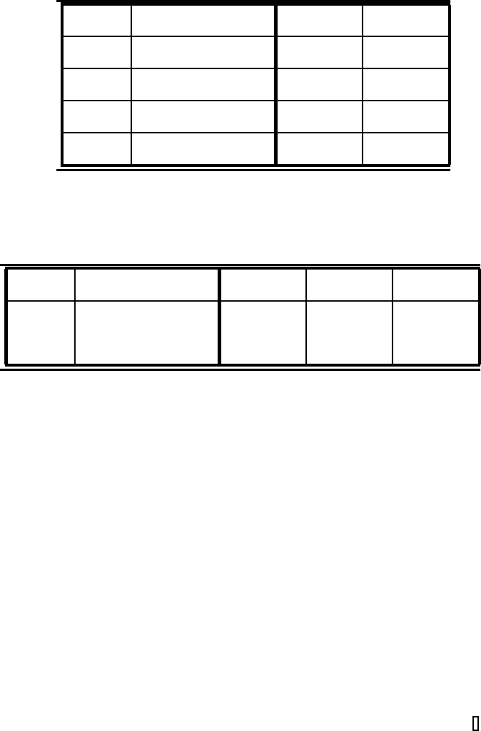
TABLE 6.7: Numerical results for the stiﬀ example with

iterative operator-splitting method and BDF3 method.

Iteration Number of err

err

steps i splitting partitions n

5 1 3.4434e-001 3.4434e-001

5 10 3.0907e-004 3.0907e-004

10 1 2.2600e-006 2.2600e-006

10 10 1.5397e-011 1.5397e-011

15 1 9.3025e-005 9.3025e-005

15 10 5.3002e-013 5.4205e-013

20 1 1.2262e-010 1.2260e-010

20 10 2.2204e-014 2.2768e-018

TABLE 6.8: Numerical results for the third example with iterative

operator-splitting method and BDF3 method with Δx =10

−2

Iteration Number of err err err

steps i splitting partitions n at x =18 at x =20 at x =22

1 10 9.8993e-002 1.6331e-001 9.9054e-002

2 10 9.5011e-003 1.6800e-002 8.0857e-003

3 10 9.6209e-004 1.9782e-002 2.2922e-004

4 10 8.7208e-004 1.7100e-002 1.5168e-005

We choose diﬀerent iteration steps and time partitions, and show the error

between the analytical and numerical solution in the supremum norm.

Figure 6.2 shows the initial solution at t

=10

, and the analytical as well

as the numerical solutions at t

end

=2·10

of the convection-diﬀusion-reaction

equation.

One result we can see is that we can reduce the error between the analyt-

ical and the numerical solution by using more iteration steps. If we restrict

ourselves to an error of 10

−4

, we obtain an eﬀective computation with three

iteration steps and ten time partitions.

REMARK 6.4 For the partial diﬀerential equations, we also need to

take into account the spatial discretization. We applied a ﬁne grid step on the

spatial discretization, such that the error of the time discretization method is

dominant. We obtain an optimal eﬃciency of the iteration steps and the time

partitions, if we use ten iteration steps and two time partitions.

Numerical Experiments 131

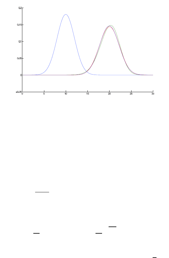
FIGURE 6.2: Initial and computed results for the third example with it-

erative splitting method and BDF3 method; the initial solution is plotted as

blue line, the iterative solution is plotted as green line, and the exact solution

is plotted as red line.

6.2.4 Fourth Example: Nonlinear Ordinary Diﬀerential

Equation

As a nonlinear diﬀerential example, we choose the Bernoulli equation:

∂u(t)

∂t

= λ

u(t)+λ

(u(t))

,t∈ [0,T], (6.20)

u(0) = 1, (6.21)

with the solution

u(t)=



(1 +

)exp(−λ

t(1 − p)) −

)



1−p

, with p =0, 1. (6.22)

We choose p =2,λ

= −1, λ

= −100, and Δx =10

−2

.Forthetimeinterval

[0,T], with T = 1, we divide in n intervals with the length τ

We apply the iterative operator-splitting method with the nonlinear

operators

A(u)=λ

u(t),B(u)=λ

(u(t))

. (6.23)

The discretization of the nonlinear ordinary diﬀerential equation is performed

with higher-order Runge-Kutta methods, precisely at least third-order meth-

ods, see also [87]. Our numerical results are presented in Table 6.9. We

choose diﬀerent iteration steps and time partitions. The error between the

analytical and numerical solution is shown with the supremum norm at time

132Decomposition Methods for Diﬀerential Equations Theory and Applications

TABLE 6.9: Numerical results for the

Bernoulli equation with iterative

operator-splitting method and BDF3 method.

Iteration Number of err

steps i splitting partitions n

2 1 7.3724e-001

2 2 2.7910e-002

2 5 2.1306e-003

10 1 1.0578e-001

10 2 3.9777e-004

20 1 1.2081e-004

20 2 3.9782e-005

T =1.0. The experiments result in showing the reduced errors for more it-

eration steps and more time partitions. Because of the time discretization

method for ODEs, we restrict the number of iteration steps to a maximum of

ﬁve. If we restrict the error bound to 10

−3

, two iteration steps and ﬁve time

partitions give the most eﬀective combination.

REMARK 6.5 For nonlinear ordinary diﬀerential equations, the ex-

act starting function is a problem. Therefore, the initialization process is

delicate and we can decrease the splitting error by more iteration steps. Due

to the linearization, we gain almost linear convergence rates. This can be

improved by a higher-order linearization, see [16], [155].

6.2.5 Fifth Example: Partial Diﬀerential Equation

In this example, we simulate a general single-species reactive transport

equation, which can be written as

+ ∇·(vu− D ∇u)=R(u)+f(x, t), in Ω × (0,T), (6.24)

u(x, t)=0, on ∂Ω × (0,T), (6.25)

u(x, 0) = u

(x), on Ω, (6.26)

where [0,T] is a time interval, x =(x

,...,x

)

∈ Ω is the space variable,

and Ω is a domain in R

(d =1, 2, or, 3). u(x, t) is the unknown population

density or concentration of the species, v ∈ R

d,+

is a divergence-free velocity

ﬁeld, D ∈ R

d,+

× R

d,+

is a diﬀusion tensor (it is assumed that elementwise

i,j

| << |v

|∀i, j ∈{1,...,d}), R(u) is a nonlinear reaction term, and u

(x)

is an initial condition.

For the reaction term, we are concerned with the

• Radioactive decay with R(u)=−au, as a linear reaction term

Numerical Experiments 133

• Bio degradation model with R(u)=au/(u + b), as a nonlinear reaction

term

The models and detailed discussions on bio degradation can be found in

[40].

We propose, based on the discretization methods and the underlying timescales,

that the convection-reaction part of the equation serves as the basis of one

operator and that the diﬀusion part and the right-hand side serve as the basis

of a second operator. Because of the splitting, the two equations can be dealt

with separately with most eﬀective discretization methods in each case. We

propose for the convection-reaction part characteristic methods and a ﬁnite

element method for the diﬀusion part.

The transport equation (6.24) can be rewritten as an abstract operator

equation:

= A(u)+B(u), (6.27)

with

A(u)=−v ·∇u + R(u), (6.28)

B(u)=∇·(D∇u)+f(x, t). (6.29)

Let N be a positive integer, τ

:= T/N as time-step, and let t

= nτ

(n =

0, 1, ··· ,N) be a uniform partition of the time period [0,T]. We split the

equation (6.24) into two equations in each small time period [t

n+1

+ v ·∇u = R(u), (6.30)

= ∇·(D∇u)+f(x, t). (6.31)

For any x ∈ Ω, the characteristic y(s; x, t

n+1

) passing through (x, t

n+1

)is

determined by

⎧

⎨

⎩

= v(y, s),s∈ (t

n+1

y(t

n+1

; x, t

n+1

)=x.

(6.32)

Let (x

∗

) be the image of exact backtracking of (x, t

n+1

). If the char-

acteristic reaches the boundary, then we use (x

∗

), where x

∗

∈ ∂Ω,t

≤

∗

≤ t

n+1

. Notice that exact tracking of characteristics is usually unavailable

in practice and we have to resort to numerical means. All commonly used

numerical methods for solving ODEs (e.g., Euler and Runge-Kutta methods),

can be applied to problem (6.32).

Along characteristics, the convection-reaction equation becomes a nonlinear

ODE:

⎧

⎨

⎩

(1)

= R(u

(1)

),t∈ (t

∗

n+1

(1)

∗

)=u

(2)

∗

(6.33)

134Decomposition Methods for Diﬀerential Equations Theory and Applications

where u

(2)

is the solution for the parabolic problem and will be explained

later. When n =0orx

∗

∈ ∂Ω, we should replace u

(2)

∗

)byu

∗

)or

the boundary condition.

Problem (6.33) can be solved numerically by for example, Euler and Runge-

Kutta methods. With a numerical solution, the nonlinearity in the reaction

term can be well resolved if R(u) is Lipschitz continuous with respect to u,

which is true for the bio degradation models and also logistic models, see [94].

The other part of the equation to solve is an initial boundary value problem

for a typical parabolic equation

⎧

⎪

⎨

⎪

⎩

(2)

= ∇·(D∇u

(2)

)+f(x, t),x∈ Ω,t∈ (t

n+1

(2)

∂Ω

=0,

(2)

(x, t

)=u

(1)

(x, t

n+1

(6.34)

This problem is conventional and can be solved by ﬁnite diﬀerence, element,

or volume methods.

Let Δx be the spatial mesh size in the numerical scheme (ﬁnite diﬀerence,

element, or volume) for solving the parabolic part (6.34), τ is the temporal

step size. Because |D| << 1, the stability condition |D|τ/Δx

≤ 1/2 is readily

satisﬁed.

6.2.5.1 Linear Reaction

To examine our method, we ﬁrst consider a two-dimensional problem with

a linear reaction, to which we can ﬁnd the exact solution. This enables us

to compare the numerical and exact solutions. In particular, we have a ro-

tating velocity v =(−4y, 4x), a constant scalar diﬀusion D>0, a linear

reaction R(u)=Ku with K being a constant, and a null source/sink (i.e.,

f ≡ 0). Assume the substance is initially normally distributed that is, the

initial condition is speciﬁed as a Gaussian hill:

(x, y)=exp



−

(x − x

)

+(y − y

)

2σ



, (6.35)

where (x

) is the center and σ>0 is the standard deviation. Then the

exact solution is given by

u(x, y, t)=

2σ

+4Dt

exp



Kt −

∗

− x

)

+(y

∗

− y

)

2σ

+4Dt



, (6.36)

where (x

∗

, 0) is the backtracking foot of the characteristic from (x, y, t)

that is,



∗

=(cos4t)x +(sin4t)y,

∗

= −(sin 4t)x +(cos4t)y.

(6.37)

Numerical Experiments 135

TABLE 6.10: Numerical results of example with linear

reaction and τ = π/8.

Mesh size Δx err

u,L

∞

err

u,L

err

u,L

1/20 1.266 ×10

−2

1.247 ×10

−4

3.138 ×10

−4

1/40 1.031 ×10

−2

5.061 ×10

−5

2.085 ×10

−4

1/50 9.984 ×10

−3

4.153 ×10

−5

1.923 ×10

−4

1/60 9.796 ×10

−3

3.613 ×10

−5

1.825 ×10

−4

For simplicity, we use a uniform triangular mesh. The second-order Runge-

Kutta (or Heun) method is used for characteristic tracking even though exact

tracking is available. The ﬁnite element solver for the parabolic part can

be implemented as a dynamic link library (DLL) which is derived from the

source code in an object ﬁnite element library (OFELI), see [162]. Therefore,

the implementation is at least only a recoding and application of established

FEM libraries and can be programmed very quickly.

For numerical runs, we choose T = π/2, Ω = [−1, 1] × [−1, 1], D =10

−4

K =0.1, (x

)=(−0.5, −0.5), and σ

=0.01. For the parabolic solver,

we use 20 micro steps within each global time-step [t

n+1

]. Accordingly, we

set the maximum number of time-steps in the characteristic tracking to 20.

Table 6.10 lists some results for the numerical solution at the ﬁnal time. We

still obtain very good numerical solutions even with large global time-steps.

6.2.5.2 Nonlinear Reaction

The second example is a simpliﬁed model for single-species bio degradation:

R(u)=au/(u + b). We consider a two-dimensional problem with a constant

velocity ﬁeld (v

)

, a scalar diﬀusion D>0, and no source/sink. The

initial condition is a normal distribution (Gaussian hill). Again we use the

parabolic solver (DLL) compiled from OFELI.

TABLE 6.11: Numerical results of

example with nonlinear reaction.

time-step τ Mesh size Δx u

min

max

0.25 1/20 0.0 1.5159

0.25 1/40 0.0 1.5176

0.25 1/60 0.0 1.5179

0.125 1/40 0.0 1.5251

0.10 1/20 0.0 1.5248

0.10 1/50 0.0 1.5268

For numerical runs, we choose T =1,Ω=[−1, 1]×[−1, 1], (v

)

=(1, 1),

136Decomposition Methods for Diﬀerential Equations Theory and Applications

D =10

−4

, a = b =1,(x

)=(−0.5, −0.5), and σ

=0.01. Table 6.11 lists

some results of the numerical solution at the ﬁnal time.

No exact solution is known for this problem. However, from Table 6.11, we

observe that the operator-splitting method is stable and keeps positivity of

the solution.

REMARK 6.6 We apply an operator-splitting method for transport

equations with nonlinear reactions. In the implementation of the proposed

method, we incorporate some existing commercial and free software compo-

nents. By integrating functionalities of existing software components, appli-

cation developers do not have to create everything from scratch.

In the numerical results, we see that the method works very well and that

we have eﬃcient computations. A simple extension of the proposed operator-

splitting method can also be made to coupled systems, see [105].

6.3 Benchmark Problems for the Spatial

Decomposition Methods:

Schwarz Waveform-Relaxation Method

In this section, we will present the benchmark problems for the spatial

decomposition method. They incorporate operator-splitting methods as well

as Schwarz waveform-relaxation methods.

6.3.1 First Example: Convection-Diﬀusion-Reaction

Equation

The problems are discretized using second-order approximations with re-

spect to the spatial variable using a regular spatial mesh with Δx = L/N ,

and backward approximations with respect to the time using τ as time-step.

The ﬁrst-order operator-splitting method (FOP) is considered to be the basic

solution algorithm for the overlapping Schwarz waveform-relaxation method

(FOPSWR). We also consider the second-order operator-splitting method

(SOP), performed as the Strang splitting method, see [185], and considered

to be the basic solution algorithm for the overlapping Schwarz waveform-

relaxation method (SOPSWR).

We consider the one-dimensional convection-diﬀusion-reaction equation given

∂

u + v∂

u − ∂

D∂

u = −λu, (6.38)

u(x, t

)=u

exact

(x, t

),u(±∞,t)=0, (6.39)