Gebali F. Analysis Of Computer And Communication Networks

Подождите немного. Документ загружается.

Chapter 3

Markov Chains

3.1 Introduction

We explained in Chapter 1 that in order to study a stochastic system we map its

random output to one or more random variables. In Chapter 2 we studied other

systems where the output was mapped to random processes which are functions of

time. In either case we characterized the system using the expected value, variance,

correlation, and covariance functions. In this chapter we study stochastic systems

that are best described using Markov processes. A Markov process is a random

process where the value of the random variable at instant n depends only on its

immediate past value at instant n −1. The way this dependence is defined gives rise

to a family of sample functions just like in any other random process. In a Markov

process the random variable represents the state of the system at a given instant

n. The state of the system depends on the nature of the system under study as we

shall see in that chapter. We will have a truly rich set of parameters that describe a

Markov process. This will be the topic of the next few chapters. The following are

the examples of Markov processes we see in many real life situations:

1. telecommunication protocols and hardware systems

2. customer arrivals and departures at banks

3. checkout counters at supermarkets

4. mutation of a virus or DNA molecule

5. random walk such as Brownian motion

6. arrival of cars at an intersection

7. bus rider population during the day, week, month, etc

8. machine breakdown and repair during use

9. the state of the daily weather

3.2 Markov Chains

If the state space of a Markov process is discrete, the Markov process is called a

Markov chain. In that case the states are labeled by the integers 0, 1, 2, etc. We will

F. Gebali, Analysis of Computer and Communication Networks,

DOI: 10.1007/978-0-387-74437-7



Springer Science+Business Media, LLC 2008

66 3 Markov Chains

be concerned here with discrete-time Markov chains since they arise naturally in

many communication systems.

3.3 Selection of the Time Step

A Markov chain stays in a particular state for a certain amount of time called the

hold time. At the end of the hold time, the Markov chain moves to another state

at random where the process repeats again. We have two broad classifications of

Markov chains that are based on how we measure the hold time.

1. Discrete-time Markov chain: In a discrete-time Markov chain the hold time as-

sumes discrete values. As a result, changes in the states occur at discrete time

values. In that case time is measured at specific instances:

t = T

, T

, ...

The spacing between the time steps need not be equal in the general case. Most

often, however, the discrete time values are equally spaced and we can write

t = nT (3.1)

n = 0, 1, 2, ... (3.2)

The time step value T depends on the system under study as will be explained

below.

2. Continuous-time Markov chain: In a continuous-time Markov chain the hold

time assumes continuous values. As a result, changes in the states occur at any

time value. The time value t will be continuous over a finite or infinite interval.

3.3.1 Discrete-Time Markov Chains

This type of Markov chains changes state at regular intervals. The time step could

be a clock cycle, start of a new day, or a year, etc.

Example 3.1 Consider a packet buffer where packets arrive at each time step with

probability a and depart with probability c. Identify the Markov chain and specify

the possible buffer states.

We choose the time step in this example to be equal to the time required to

receive or transmit a packet (transmission delay). At each time step we have two

independent events: packet arrival and packet departure. We model the buffer as a

Markov chain where the states of the system indicate the number of packets in the

buffer. Assuming the buffer size is B, then the number of states of the buffer is B +1

as identified in Table 3.1.

3.3 Selection of the Time Step 67

Table 3.1 States of buffer

occupancy

State Significance

0bufferisempty

1 buffer has one packet

2 buffer has two packets

B buffer has B packets (full)

Example 3.2 Suppose that packets arrive at random on the input port of a router

at an average rate λ

(packets/s). The maximum data rate is assumed to be σ

(packets/s), where σ>λ

. Study the packet arrival statistics if the port input is

sampled at a rate equal to the average data rate λ

The time step (seconds) is chosen as

T =

In one time step we could receive 0, 1, 2, ..., N packets; where N is the maxi-

mum number of packets that could arrive

N =σ × T =



where the ceiling function f (x) =xgives the smallest integer larger than or equal

to x.

The statistics for packet arrival follow the binomial distribution and the proba-

bility of receiving k packets in time T is

p(k) =





N−k

where a is the probability that a packet arrives and b = 1 −a. Our job in almost all

situations will be to find out the values of the parameters N, a, and b in terms of the

given data rates.

The packet arrival probability a could be obtained using the average value of the

binomial distribution. The average input traffic N

(in) is given from the binomial

distribution by

(in) = Na

But N

(in) is also determined by the average data rate as

(in) = λ

× T = 1

68 3 Markov Chains

From the above two equations we get

a =

≤

Example 3.3 Consider Example 3.2 when the input port is sampled at the rate σ .

The time step is now given by



In one time step we get either one packet or no packets. There is no chance to get

more than one packet in one time step since packets cannot arrive at a rate higher

than σ . Therefore, the packet arrival statistics follow the Bernoulli distribution. For

a time period t, the average number of packets that arrives is

(in) = λ

From the Bernoulli distribution that average is given by

(in) = a



The fraction on RHS indicates the number of time steps spanning the time period

t. From the above two equations we get



= λ



3.4 Memoryless Property of Markov Chains

In a discrete-time Markov chain, the value of the random variable S(n) represents the

state of the system at time n. The random variable S(n) is a function of its immediate

past value—i.e. S(n) depends on S(n −1). This is referred to as the Markov property

or memoryless property of the Markov chain where the present state of the system

depends only on its immediate past state [1, 2]. Alternatively, we can say that the

Markov property of the Markov chain implies that the future state of the system

depends only on the present sate and not on its past states [3].

The probability that the Markov chain is in state s

at time n is a function of its

past state s

at time n − 1 only. Mathematically, this statement is written as

[

S(n) = s

]

= f





(3.3)

3.5 Markov Chain Transition Matrix 69

3 4

0 1 2

Fig. 3.1 The occupancy states of a buffer of size four and the possible transitions between the

states

for all i ∈ S and j ∈ S where S is the set of all possible states of the system.

Transition from a state to the next state is determined by a transition probability

only with no regard to how the system came to be in the present state. Many commu-

nication systems can be modeled as Markov or memoryless systems using several

techniques such as introducing extra transitions, defining extra states, and adjusting

the time step value. This effort is worthwhile since the memoryless property of a

Markov chain will result in a linear system that can be easily studied.

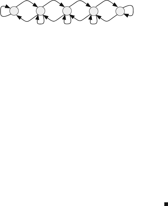
Example 3.4 Consider a data buffer in a certain communication device such as a

network router for example. Assume the buffer could accommodate at most four

packets. We say the buffer size is B = 4. Identify the states of this buffer and show

the possible transitions between states assuming at any time step at most one packet

can arrive or leave the buffer. Finally explain why the buffer could be studied using

Markov chain analysis.

Figure 3.1 shows the occupancy states of a buffer of size four and the possible

transitions between the states. The buffer could be empty or it could contain 1, 2, 3,

or 4 packets. Furthermore, the assumptions indicate that the size of the buffer could

remain unchanged or it could increase or decrease by one.

The transition from one state to another does not depend on how the buffer

happened to be in the present state. Thus the system is memoryless and could be

modeled as a Markov chain.

3.5 Markov Chain Transition Matrix

Let us define p

(n) as the probability of finding our system in state i at time step

n given that the past state was state j. We equate p

to the conditional probability

that the system is in state i at time n given that it it was in state j at time n − 1.

Mathematically, we express that statement as follows.

(n) = p

[

S(n) = i

S(n −1) = j

]

(3.4)

The situation is further simplified if the transition probability is independent of

the time step index n. In that case we have a homogeneous Markov chain, and the

above equation becomes

= p

[

S(n) = i

S(n −1) = j

]

(3.5)

70 3 Markov Chains

Let us define the probability of finding our system in state i at the nth step as

(n) = p

[

X(n) = i

]

(3.6)

where the subscript i identifies the state and n denotes the time step index. Using

(3.4), we can express the above equation as

(n) =



j=1

×s

(n − 1) (3.7)

where we assumed the number of possible states to be m and the indices i and j

lie in the range 1 ≤ i ≤ m and 1 ≤ j ≤ m. We can express the above equation in

matrix form as

s(n) = Ps(n − 1) (3.8)

where P is the state transition matrix of dimension m × m

P =

⎡

⎢

⎣

··· p

1,m

··· p

2,m

m,1

m,2

··· p

m,m

⎤

⎥

⎦

(3.9)

and s(n)isthedistribution vector (or state vector) defined as the probability of the

system being in each state at time step n:

s(n) =



(n) s

(n) ··· s

(n)



(3.10)

The component s

(n) of the distribution vector s(n) at time n indicates the proba-

bility of finding our system in state s

at that time. Because it is a probability, our

system could be in any of the m states. However, the probabilities only indicate

the likelihood of being in a particular state. Because s describes probabilities of all

possible m states, we must have



i=1

(n) = 1 n = 0, 1, 2, ··· (3.11)

We say that our vector is normalized when it satisfies (3.11). We call such a

vector a distribution vector. This is because the vector describes the distribution of

probabilities among the different states of the system.

Soon we shall find out that describing the transition probabilities in matrix form

leads to great insights about the behavior of the Markov chain. To be specific, we

will find that we are interested in more than finding the values of the transition

3.5 Markov Chain Transition Matrix 71

probabilities or entries of the transition matrix P. Rather, we will pay great attention

to the eignevalues and eigenvectors of the transition matrix.

Since the columns of P represent transitions out of a given state, the sum of each

column must be one since this covers all the possible transition events out of the

state. Therefore we have, for all values of j,



i=1

= 1 (3.12)

The above equation is always valid since the sum of each column in P is unity.

For example, a 2×2 transition matrix P would be set up as in the following diagram:

Present state

↓

Next state

←

⎡

⎣

⎤

⎦

The columns represent the present state while the rows represent the next state.

Element p

represents the transition probability from state j to state i. For example,

is the probability that the system makes a transition from state s

to state s

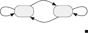
Example 3.5 An on–off source is often used in telecommunications to simulate

voice traffic. Such a source has two states: The silent state s

where the source

does not send any data packets and the active state s

where the source sends one

packet per time step. If the source were in s

, it has a probability s of staying in that

state for one more time step. When it is in state s

, it has a probability a of staying

in that state. Obtain the transition matrix for describing that source.

The next state of the source depends only on its present state. Therefore, we can

model the state of the source as a Markov chain. The state diagram for such source

is shown in Fig. 3.2 and the transition matrix is given by

P =



s 1 −a

1 −sa



Fig. 3.2 Transition diagram

for an on–off source

1-s

1-a

Active

State

Silent

State

72 3 Markov Chains

Fig. 3.3 AMarkovchain

involving three states

3/4

1/4

3/4

1/4

1/2

Colwood

Langford

Sooke

Example 3.6 Assume that the probability that a delivery truck moves between three

cities at the start of each day is shown in Fig. 3.3. Write down the transition

matrix and the initial distribution vector assuming that the truck was initially in

Langford.

We assume the city at which the truck is located is the state of the truck. The next

state of the truck depends only on its present state. Therefore, we can model the state

of the truck as a Markov chain. We have to assign indices to replace city names. We

chose the following arbitrary assignment, although any other state assignment will

work as well.

City State index

Colwood 1

Langford 2

Sooke 3

Based on the state assignment table, the transition matrix is given by

⎡

⎣

01/41/4

3/401/4

1/43/41/2

⎤

⎦

The initial distribution vector is given by

(

)



010



Example 3.7 Assume an on–off data source that generates equal length packets with

probability a per time step. The channel introduces errors in the transmitted packets

such that the probability of a packet is received in error is e. Model the source using

Markov chain analysis. Draw the Markov chain state transition diagram and write

the equivalent state transition matrix.

3.5 Markov Chain Transition Matrix 73

The Markov chain model of the source we use has four states:

State Significance

1 Source is idle

2 Source is retransmitting a frame

3 Frame is transmitted with no errors

4 Frame is transmitted with an error

Since the next state of the source depends only on its present state, we can model

the source using Markov state analysis.

Figure 3.4 shows the Markov chain state transition diagram. We make the fol-

lowing observations:

• The source stays idle (state s

) with probability 1 −a.

• Transition from s

to s

occurs under two conditions: the source is active and no

errors occur during transmission.

• Transition from s

to s

occurs under two conditions: the source is active and an

error occurs during transmission.

• Transition from s

to s

occurs under only one condition: no errors occur.

The associated transition matrix for the system is given by

P =

⎡

⎢

⎣

1 −a 010

0001

a(1 −e)1−e 00

ae e 00

⎤

⎥

⎦

Example 3.8 In an ethernet network based on the carrier sense multiple access with

collision detection (CSMA/CD), a user requesting access to the network starts trans-

mission when the channel is not busy. If the channel is not busy, the user starts

Fig. 3.4 State transition

diagram for transmitting a

packet over a noisy channel

1-a

a (1-e)

1-e

a e

74 3 Markov Chains

transmitting. However, if one or more users sense that the channel is free, they will

start transmitting and a collision will take place. If a collision from other users is

detected, the user stops transmitting and returns to the idle state gain. In other words,

we are not adopting any backoff strategies for simplicity in this example.

Assume the following probabilities:

Probability all users are idle

Probability only one user is transmitting

1 −u

−u

Probability two or more users are transmitting

(a) Justify using Markov chain analysis to describe the behavior of the channel or

communication medium.

(b) Select a time step size for a discrete-time Markov chain model.

transition probabilities.

(a) A user in that system will determine its state within a time frame of twice the

propagation delay on the channel. Therefore, the current state of the channel

or communication medium and all users will depend only on the actions of

the users in time frame of one propagation delay only. Thus our system can be

described as a Markov chain.

(b) The time step T we can choose is twice the propagation delay. Assume packet

transmission delay requires n time steps where all packets are assumed to have

equal lengths.

(1) i: idle state

(2) t: transmitting state

(3) c: collided state

Fig. 3.5 Markov chain state

transition diagram for the

CSMA/CD channel

Idle

Collided

Transmitting

1-u

-u

...