Drake G.W.F. (editor) Handbook of Atomic, Molecular, and Optical Physics

Подождите немного. Документ загружается.

Relativistic Atomic Structure 22.5 Spherical Symmetry 337

and inserting into (22.85), resulting in a hierarchy of

equations



Ω

(1)

, H



P = (V − PV )P = QVP ,



Ω

(2)

, H



P =



QVΩ

(1)

−Ω

(1)



P ,

and so on, with H

(n)

eff

= PVΩ

(n−1)

22.4.5 Perturbation Theory: Algorithms

The techniques of QED perturbation theory of

Sect. 22.3.4 can be utilized to give computable expres-

sions for perturbation calculations order by order. They

exploit the second quantized representation of opera-

tors of Sect. 22.4.1 along with the use of diagrams to

express the contributions to the wave operator and the

energy as sums over virtual states. The use of Wick’s

theorem to reduce products of normally-ordered opera-

tors, and the linked-diagram or linked-cluster theorem

are explained in Lindgren’s article [22.17]andChapt.5.

Further references and discussion of features which

can exploit vector-processing and parallel-processing

computer architectures may be found in [22.18].

The theory can also be recast so as to sum certain

classes of terms to completion. This depends on the

possibility of expressing the wave operator as a normally

ordered exponential operator

Ω ={exp S}=1 +{S}+

}+··· ,

where the normally ordered operator S is known as the

cluster operator. Expanding S order by order leads to the

coupled cluster expansion (see also Chapts. 5 and 27).

22.5 Spherical Symmetry

A popular starting point for most calculations in atomic

and molecular structure is the independent particle cen-

tral ﬁeld approximation. This assumes that the electrons

move independently in a potential ﬁeld of the form

(x) =

φ(r), r =|x|;

(x) = 0 , i = 1, 2, 3 . (22.86)

Clearly φ(r) is left unchanged by any rotation about the

origin, r = 0, but transforms as the component A

(x)

of a 4-vector under other types of Lorentz and Poincaré

transformation such as boosts or translations. However,

solutions in central potentials of this form have a simple

form which is convenient for further calculation.

With this restriction on the 4-potential, Dirac’s

Hamiltonian becomes



cα · p+eφ(r) +βm



(22.87)

Consider stationary solutions with energy E satisfying

(x) = Eψ

(x).

Since

is invariant with respect to rotation about

r = 0, it commutes with the generators J

, J

men-

tioned in Sect. 22.1.1, corresponding to components of

the total angular momentum j of the electron, usually

decomposed into an orbital part l and a spin part s,

j = l+s

(22.88)

where

= i

jkl

∂

, j = 1, 2, 3



jkl

, j = 1, 2, 3 .

22.5.1 Eigenstates of Angular Momentum

We can construct simultaneous eigenstates of the op-

erators j

and j

by using the product representation

(l)

× D

(1/2)

of the rotation group SO(3), which is

reducible to the Clebsch–Gordan sum of two irreps

(l+1/2)

⊕D

(l−1/2)

. (22.89)

We construct a basis for each irrep from products of ba-

sisvectorsforD

(1/2)

and D

(l)

respectively. D

(1/2)

a 2-dimensional representation spanned by the simulta-

neous eigenstates φ

of s

and s

, s

= σφ

,σ=±

for which we can use 2-rowed vectors

1/2





,φ

−1/2





The representation D

(l)

is (2l +1)-dimensional; its basis

vectors can be taken to be the spherical harmonics



(θ, ϕ) |m =−l, −l +1,... ,l



Part B 22.5

338 Part B Atoms

so that

(θ, ϕ) = l(l +1)

(θ, ϕ) ,

(θ, ϕ) = m Y

(θ, ϕ) .

We shall assume that spherical harmonics satisfy the

standard relations

(θ, ϕ) =[l(l+1)−m(m ±1)]

1/2

m±1

(θ, ϕ) ,

where l

±l

,sothat

(θ, ϕ) =



2l +1

4π



1/2

(θ, ϕ) ,

(θ, ϕ) = (−1)



(l −m)!

(l +m)!



1/2

(θ) e

imϕ

if m ≥0 ,

−m

(θ, ϕ) = (−1)

(θ, ϕ)

∗

. (22.90)

Basis functions for the representations D

with

j = l ±

have the form (The order of coupling is sig-

niﬁcant, and great confusion results from a mixing

of conventions. Here we couple in the order l, s, j.

The same spin-angle functions are obtained if we

use the order s, l, j but there is a phase difference

(−1)

l−j+1/2

= (−1)

(1−a)/2

. You have been warned!)

j,m,a

(θ, ϕ)



l, m −σ,

,σ

, j, m

m−σ

(θ, ϕ)φ

(22.91)

where l, m −σ,

,σ|l,

, j, m is a Clebsch–Gordan

coefﬁcient with

l = j −

a, a =±1,

m =−j, −j +1,... , j −1, j .

Inserting explicit expressions for the Clebsch–Gordan

coefﬁcients gives

j,m,−1

(θ, ϕ) =







−

j+1−m

2 j+2

1/2

m−1/2

j+1/2

(θ, ϕ)

j+1+m

2 j+2

1/2

m+1/2

j+1/2

(θ, ϕ)







j,m,1

(θ, ϕ) =







j+m

2 j

1/2

m−1/2

j−1/2

(θ, ϕ)

j−m

2 j

1/2

m+1/2

j−1/2

(θ, ϕ)







(22.92)

The vectors (22.92) satisfy

j,m,a

= j( j +1)χ

j,m,a

, s

j,m,a

=l(l +1)χ

j,m,a

, l = j −

a, a =±1 .

(22.93)

The parity of the angular part is given by (−1)

, with the

two possibilities distinguished by means of the operator



=−( j

−l

−s

+1) =−(2s· l +1) (22.94)

so that



j,m,a



j,m,a

, k



=−



j +



a, a =±1 .

The basis vectors are orthonormal on the unit sphere

with respect to the inner product

(χ



|χ

jma

)



†



(θ, ϕ)χ

j,m,a

(θ, ϕ) sin θ dθ dϕ

= δ



, j



. (22.95)

22.5.2 Eigenstates of Dirac Hamiltonian

in Spherical Coordinates

Eigenstates of Dirac’s Hamiltonian (22.87) in spheri-

cal coordinates with a spherically symmetric potential

V(r) = eφ(r),

(r) = Eψ

(r), (22.96)

are also simultaneous eigenstates of j

,of j

and of the

operator

K =





0 −K



(22.97)

where K



is deﬁned in (22.94) above. Denote the cor-

responding eigenvalues by j, m and κ,where

κ =±



j +



(22.98)

Then the simultaneous eigenstates take the form

Eκm

(r) =



Eκ

(r)χ

κ,m

(θ, ϕ)

Eκ

(r)χ

−κ,m

(θ, ϕ)



(22.99)

where κ =−( j +1/2)a is the eigenvalue of K



,andthe

notation χ

κ,m

replaces the notation χ

j,m,a

used previ-

ously in (22.91). The factor i in the lower component

Part B 22.5

Relativistic Atomic Structure 22.5 Spherical Symmetry 339

ensures that, at least for bound states, the radial am-

plitudes P

Eκ

(r), Q

Eκ

(r) can be chosen to be real. This

decomposition into radial and angular factors exploits

the identity

σ · p



F(r)

κ,m

(θ, ϕ)



= i



κF



−κ,m

(θ, ϕ) (22.100)

and gives a reduced eigenvalue equation





− E +V −c

−

−mc

− E +V







Eκ

(r)

Eκ

(r)



= 0 .

(22.101)

Angular Density Distributions

It is a remarkable fact that the angular density distribu-

tion

κ,m

(θ, ϕ) = χ

κ,m

(θ, ϕ)

†

κ,m

(θ, ϕ) , (22.102)

where m =−j, −j +1,... , j −1, j,isindependent of

the sign of κ; the equivalence of

j+1/2,m

(θ, ϕ) =

4π

( j −m)!

( j +m)!



( j −m +1)

m−1/2

j+1/2

(µ)

m+1/2

j+1/2

(µ)



and

−( j+1/2),m

(θ, ϕ) =

4π

( j −m)!

( j +m)!



( j +m)

m−1/2

j−1/2

(µ)

m+1/2

j−1/2

(µ)



where µ =cos θ, was demonstrated by Hartree [22.19].

Angular densities for the lowest |κ| values are given

in Table 22.1. The corresponding nonrelativistic angular

densities

l,m

(θ, ϕ)

2l +1

4π

(l −m)!

(l +m)!

|m|

(µ)

;

are listed in Table 22.2.

Radial Density Distributions

The probability density distribution ρ

Eκm

(r) associated

with the stationary state (22.99)isgivenby

E,κ,m

(r) =



E,κ

(r)|

κ,m

(θ, ϕ)

+|Q

E,κ

(r)|

−κ,m

(θ, ϕ)



. (22.103)

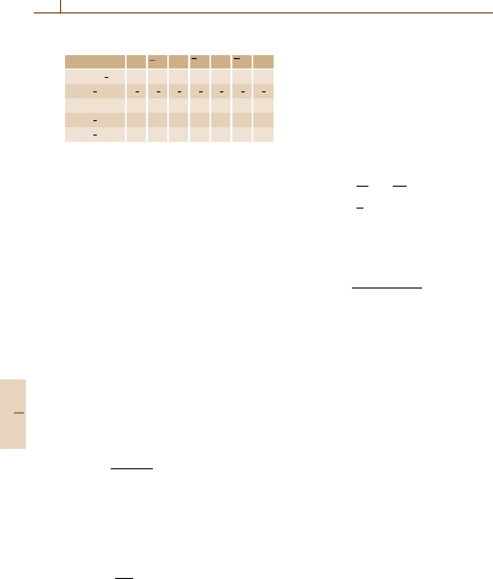
Table 22.1 Relativistic angular density functions

|κ| |m| 4π A

|κ|,m

(θ,ϕ)

sin

(1 +3cos

θ)

sin

θ(1 +15 cos

θ)

(3cos

θ −1)

+3sin

θ cos

Table 22.2 Nonrelativistic angular density functions

l |m| 4π A

l,m

(θ,ϕ)

0 0 1

1 1

sin

0 3cos

2 2

sin

θ cos

(3cos

θ −1)

Since A

κ,m

does not depend on the sign of κ, the angular

part can be factored so that

E,κ,m

(r) =

E,κ

(r)

|κ|,m

(θ, ϕ) ,

where

E,κ

(r) =



E,κ

(r)|

+|Q

E,κ

(r)|



(22.104)

deﬁnes the radial density distribution.

Subshells in j–j Coupling

The notion of a subshell depends on the observation that

the set {ψ

E,κ,m

, m =−j,... , j} haveacommonradial

density distribution. The simplest atomic model is one

in which the electrons move independently in a mean

ﬁeld central potential. Since



m=−j

E,κ,m

(r) =

2 j +1

4π

E,κ

(r)

, (22.105)

a state of 2 j +1 independent electrons, with one in

each member of the set {ψ

E,κ,m

, m =−j,... , j},has

a spherically symmetric probability density. If E be-

longs to the point spectrum of the Hamiltonian, then

(22.105) gives a distribution localized in r,andwere-

fer to the states {E,κ,m}, m =−j,... , j as belonging

to the subshell {E,κ}.

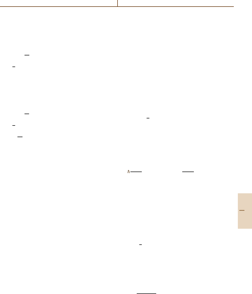
The notations in use for Dirac central ﬁeld states

are set out in Table 22.3.Herel is associated with the

orbital angular quantum number of the upper pair of

Part B 22.5

340 Part B Atoms

Table 22.3 Spectroscopic labels and angular quantum num-

bers

Label: s p p d d f f

κ =−



j +



−1 +1 −2 +2 −3 +3 −4

j = l +

a 1 −1 1 −1 1 −1 1

l = j −

a 0 1 1 2 2 3 3

l = j +

a 1 0 2 1 3 2 4

components and

l with the lower pair. Note the useful

equivalence

κ(κ +1) =l(l +1).

Deﬁning

κ := −κ we have also

κ(

κ +1) =

l +1).

22.5.3 Radial Amplitudes

Textbooks on quantum electrodynamics usually contain

extensive discussions of the formalism associated with

the Dirac equation but rarely go beyond the treatment of

the hydrogen atom Chapt. 10. Greiner’s textbook [22.4]

is an honorable exception, with many worked exam-

ples. A more exhaustive list of problems in which exact

solutions are known is contained in [22.20]; it is par-

ticularly rich in detail about equations of motion and

Green’s functions in external electromagnetic ﬁelds of

various conﬁgurations; coherent states of relativistic par-

ticles; charged particles in quantized plane wave ﬁelds. It

also incorporates discussion of extensions of the Dirac

equations due to Pauli which include explicit interac-

tion terms arising from anomalous magnetic or electric

moments.

Atoms and molecules with more than one electron

are not soluble analytically so that numerical models

are needed to make predictions. The solutions are sen-

sitive to boundary conditions on which we focus in this

section. For large r, solutions of (22.101) can be found

proportional to exp(±λr),where

λ =+

− E

. (22.106)

Thus λ is real when −c

≤ E ≤ c

,andpure imaginary

otherwise.

Singular Point at r = 0

Singularities of the nuclear potential near r = 0have

a major inﬂuence on the nature of solutions of the Dirac

equation. Suppose that the potential has the form

V(r) =−

Z(r)

(22.107)

so that Z(r) is the effective charge seen by an electron

at radius r from the nuclear center. The dependence of

Z(r) on r may reﬂect the ﬁnite size of the nuclear char ge

distribution, so far treated as a point, or the screening due

to the environment. Assume that Z(r) can be expanded

in a power series of the form

Z(r) = Z

+ Z

r +Z

+··· (22.108)

in a neighborhood of r = 0. This property characterizes

a number of well-used models

1. Point nucleus: Z

= 0; Z

= 0, n > 0.

2. Uniform nuclear charge distribution:

V(r) =











−



1 −



, 0 ≤ r ≤ a ,

−

, r > a .

(22.109)

This gives the expansion Z

=−3Z/2a, Z

= 0,

=+Z/2a

, Z

= 0forn > 2whenr ≤ a.

3. Fermi distribution: The nuclear charge density has

the form

nuc

(r) =

1 +exp[(r −a)/d]

where ρ

is chosen so that the total charge on the

nucleus is Z.

Other nuclear models, reﬂecting the density distribu-

tions deduced from nuclear scattering experiments, can

be found in the literature.

Series Solutions Near r = 0

Any solution for the radial amplitudes of Dirac’s equa-

tion in a central potential

u(r) =



P(r)

Q(r)



(22.110)

with radial density

D(r) = P

(r) +Q

(r),

can be expanded in a power series near the singular point

at r = 0 in the form

u(r) = r



r +u

+···



, (22.111)

where





, k = 1, 2,...

and γ, p

, q

are constants which depend on the nuclear

potential model.

Part B 22.5

Relativistic Atomic Structure 22.5 Spherical Symmetry 341

Point Nuclear Models

For a Coulomb singularity, Z

= 0, the leading coefﬁ-

cients satisfy

−Z

+c(κ −γ)q

= 0 ,

c(κ +γ) p

− Z

= 0 , (22.112)

so that

γ =±

(

−

c(κ −γ)

c(κ +γ)

. (22.113)

Finite Nuclear Models

Finite nuclear models, for which Z

= 0, have no sin-

gularity in the potential at r = 0. The indicial equation

(22.113) reduces to γ =±|κ|, so that for κ<0,

P(r) = p

l+1



l+3



(22.114)

Q(r) = q

l+2



l+4



(22.115)

with

/ p



E −mc

+ Z

)

[c(2l +3)] ,

= p

= 0 ,

and for κ ≥ 1,

P(r) = p

l+1



l+3



(22.116)

Q(r) = q



l+2



(22.117)

with

=−



E −mc

+ Z

)

[c(2l +1)] ,

= q

= 0 .

In both cases the solutions consist of either purely even

powers or purely odd powers of r, contrasting strongly

with the point nucleus case, where both even and odd

powers are present in the series expansion.

The Nonrelativistic Limit

For a solution linked to a nonrelativistic state with orbital

angular momentum l, one expects the nonrelativistic

limit

P(r) = O



l+1



, c →∞.

The limiting behavior reveals some signiﬁcant features.

Finite nuclear models.

The behavior is entirely regular:

P(r) = O



l+1



, Q(r) = O



−1



→ 0 .

Point nuclear models.

Since

γ =|κ|−

|κ|

+··· ,

(22.113) shows that the leading coefﬁcient p

vanishes

in the limit so that,

P(r) ≈ p

l+1



1 +O







, when κ ≥ 1, l = κ.

(22.118)

All higher powers of odd relative order vanish in the limit

for both components. The behavior in the case κ<0is

entirely regular.

22.5.4 Square Integrable Solutions

Square integrable solutions require

E,κ

(r)dr to be

ﬁnite; since the solutions are smooth, except possibly

near the singular endpoints r → 0andr →∞, we focus

on the behavior at the endpoints:

r →∞

For real values of λ the condition

∞



E,κ

(r)dr < ∞ , 0 < R < ∞ ,

requires that P

Eκ

(r), Q

Eκ

(r) are proportional to

exp(−λr) with λ>0.

This means that bound states can only exist when

E lies in the interval −c

≤ E ≤c

. Outside this interval

solutions are necessarily of scattering type and so

∞



E,κ

(r)dr

diverges when |E| > c

r → 0

This limit requires





E,κ

(r)dr < ∞, R



> 0 .

Part B 22.5

342 Part B Atoms

Since D

E,κ

(r) ∼r

±2γ

as r → 0, this condition holds

when ±γ>−

. Only the solution with γ>0 satis-

ﬁes the condition when |γ | >

,orZ <α

−1

−1/4,

and the solution with γ<0 must be disregarded. This

corresponds to the limit point case of a second-order dif-

ferential operator [22.21]. In the special case |κ|=1or

j =

this limits Z to be smaller than c

√

3/2 ≈ 118.6.

For Z > c

√

3/2, both solutions are square integrable

near the origin (the limit circle case) and the differential

operator is no longer essentially self-adjoint.

The Coulomb potential must have a ﬁnite expecta-

tion for any physically acceptable solution, so that we

also require





E,κ

(r)

< ∞, R



> 0 .

This is always satisﬁed by the solution with γ>0for

all |Z| <α

−1

|κ|, but not by the solution with γ<0. Im-

posing this condition restores essential self-adjointness

(on a restricted domain) for 118 < Z ≤ 137.

22.5.5 Hydrogenic Solutions

The wave functions for hydrogenic solutions of Dirac’s

equation are presented in Sect. 22.8.2. Here we note

some properties of hydrogenic solutions that reveal

dynamical effects of relativity in the absence of screen-

ing by orbital electrons. In this case Z

= Z, Z

= 0,

n > 0. When −c

< E < c

we have bound states. The

parameter λ,(22.106), can conveniently be written

λ = Z/N ,

(22.119)

so that rearranging (22.106)gives

E =+c

(

1 −

, (22.120)

essentially equivalent to Sommerfeld’s ﬁne structure for-

mula. In the formal nonrelativistic limit, c →∞,we

have

E = c

−

+O(1/c

)

so that N is closely related to the principal quantum

number, n, appearing in the Rydberg formula. As in

Sect. 22.8.2, we write ρ =2λr.

Deﬁne the inner quantum number

=−a =−γ +

, n

= 0, 1, 2,... .

Substitute for E from (22.120)toget

N =



+γ)

+α



1/2



−2n

(|κ|−γ)



1/2

, (22.121)

where n = n

+|κ| is the principal quantum number,

the exact equivalent of the principal quantum num-

ber of the nonrelativistic state to which the Dirac

solution reduces in the limit c →∞. With this nota-

tion, the radial amplitudes for bound hydrogenic states

are

Eκ

(r)

= N

Eκ

(c +E/c)

1/2

−ρ/2



−n

M(−n

+1,

2γ +1;ρ) + (N −κ)M(−n

, 2γ +1;ρ)



(22.122)

Eκ

(r)

= N

Eκ

(c −E/c)

1/2

−ρ/2



−n

M(−n

+1,

2γ +1;ρ) − (N −κ)M(−n

, 2γ +1;ρ)



(22.123)

where

Eκ



αZ

(N −κ)

Γ(2γ +n

+1)

![Γ(2γ +1)]



1/2

is the normalization constant. For deﬁnitions of

the conﬂuent hypergeometric functions M(a, b;c;z)

see [22.22, Sect. 13.1].

Table 22.4 lists expectation values of simple pow-

ers of the radial variable ρ = 2Zr/N from [22.23]

Table 22.4 Radial moments ρ



s Nonrelativistic Relativistic

2 2n

[5n

+1 2



(5N

−2κ

(N )

−3l(l +1)] +N

(1−γ

) −3κN

R(N )



1 3n

−l(l +1) −κ +(3N

−κ

)R(N )

0 1 1

−1

nγ +(|κ|−γ)|κ|

2γN

−2

(2l +1)

R(N )

2γ

(2γ −sgnκ)

−3

l(l+1)(2l+1)

+2γ

−3N

κR(N )

γ(γ

−1)(4γ

−1)

R(N ) =

1 − Z

Part B 22.5

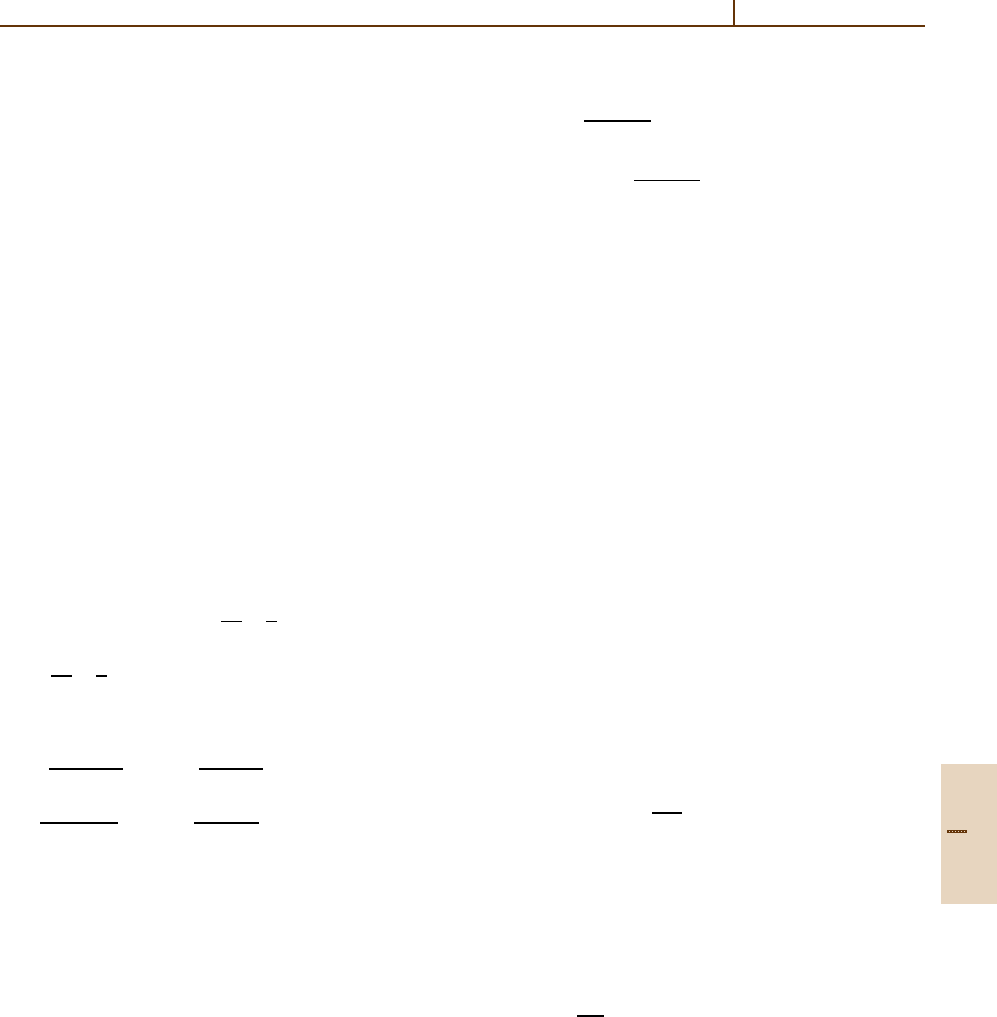
Relativistic Atomic Structure 22.5 Spherical Symmetry 343

and [22.24]. Simple algebra, using the inequalities

γ<|κ| and N < n, yields the inequality

ρ



nκ

< ρ



, s > 0 ;

the inequality is reversed for s < 0. In the same way, it is

easy to deduce that relativistic hydrogenic eigenvalues

lie below the nonrelativistic eigenvalues



nκ

<

Thus, in the absence of screening, Dirac orbitals both

contract and are stabilized with respect to their nonrela-

tivistic counterparts. The relativistic and nonrelativistic

expectation values approach each other as the relativistic

coupling constant, Z/c =αZ →0. This formal nonrela-

tivistic limit is approached as α → 0orc →∞,inwhich

the speed of light is regarded as inﬁnite.

22.5.6 The Free Electron Problem

in Spherical Coordinates

The radial equation (22.101) for the free electron

( V(r) = 0) gives a pair of ﬁrst order ordinary differential

equations

(mc

− E)P

Eκ

(r) = c



−



Eκ

(r),





Eκ

(r) =



+ E



Eκ

(r), (22.124)

from which we deduce that

Eκ

(r)



−

κ(κ +1)



Eκ

(r) = 0 ,

Eκ

(r)



−

κ(

κ +1)



Eκ

(r) = 0 ,

(22.125)

where p

= m

−E

= p. p and the angular quan-

tum numbers κ and

κ are associated respectively with the

upper and lower components. These are deﬁning equa-

tions of Riccati–Bessel functions [22.22, Sect. 10.1.1]

of orders l and

l respectively, where

κ(κ +1) =l(l +1),

κ(

κ +1) =

l +1).

Thus the solutions of (22.125) are functions of the

variable x = pr of the form

Eκ

(r) = Ax f

(x), Q

Eκ

(r) = Bx f

(x),

where the ratio of A and B is determined by (22.124)

and where f

(x) is a spherical Bessel function of the

ﬁrst, second or third kind [22.22, Sect. 10.1.1]. Thus

Eκ

(r) = N



E +mc

πE



1/2

(x ),

Eκ

(r) = N sgn(κ)



E −mc

πE



1/2

(x ).

(22.126)

Equations (22.124) require that Riccati–Bessel solu-

tions of the same type be chosen for both components.

The possibilities are:

Standing Waves

The two solutions of the same type are f

(x) =

(x), f

(x) = y

(x).The j

(x) are bounded everywhere,

including the singular points x = 0, x →∞and have

zeros of order l at x = 0. The y

(x ) are bounded at inﬁnity

but have poles of order l +1atx = 0.

Progressive Waves

The spherical Hankel functions (functions of the third

kind) are linear combinations

(1)

(x) = j

(x) +iy

(x), h

(2)

(x) = j

(x) −iy

(x).

Recalling that p is real if and only if |E| > mc

,wesee

that h

(1)

(x), h

(2)

(x) are bounded as x →∞and have

poles of order l +1atx =0. Notice that when |E|< mc

which does not occur for a free particle, p becomes pure

imaginary and no solution exists which is ﬁnite at both

singular points.

The normalization constant N can be determined by

using the well-known result

∞



( pr) j

( p



r)r

dr =

δ( p − p



The choice N = 1 ensures that

∞





†

Eκ

(r)P



(r)+Q

†

Eκ

(r)Q



(r)



dr =δ(p−p



Noting that

δ(E − E



) =

δ( p − p



and dp/ dE = c

p/E gives

∞





†

Eκ

(r)P



(r)+Q

†

Eκ

(r)Q



(r)



dr =δ(E−E



when N =



|E|/c



1/2

Part B 22.5

344 Part B Atoms

22.6 Numerical Approximation of Central Field Dirac Equations

The main drive for understanding methods of numerical

approximation of solutions of Dirac’s equation comes

from their application to many-electron systems. Ap-

proximate wave functions for atomic or molecular states

are usually constructed from products of one-electron

orbitals, and their determination exploits knowledge

gained from the treatment of one-electron problems.

Whilst the numerical methods described here are strictly

one-electron in character, extension to many-electron

problems is relatively straightforward.

22.6.1 Finite Differences

The numerical approximation of eigensolutions of the

ﬁrst order system of differential equations (22.101)



Eκ

(r)

Eκ

(r)







+V(r) −c

−

−mc

+V(r)







Eκ

(r)

Eκ

(r)



(22.127)

can be achieved by more or less standard ﬁnite differ-

ence methods given in texts such as [22.25]. For states

in either continuum, E > mc

or E < −mc

, the calcu-

lation is completely speciﬁed as an initial value problem

for a prescribed value of E starting from power series

solutions in the neighborhood of r = 0. Solutions of this

sort exist for all values of (complex) E except at the

bound eigensolutions in the gap −mc

< E < mc

.For

bound states, the calculation becomes that of a two-point

boundary value problem in which the eigenvalue E has

to be determined iteratively along with the numerical

solution. We concentrate on the latter, which is more

involved.

It is convenient to write



nκ

= E

nκ

−mc

, (22.128)

so that  approaches the nonrelativistic eigenvalue in the

limit c →∞. For the one-electron problem, (22.101)

can be written in the general form



r +W(s)



u(s) = χ(s)

(22.129)

where u(s) and χ(s) are two-component vectors, such

that

u(s) =



P(s)

Q(s)



, J =



−10



W(s) =



−rV(r) −cκ

−cκ 2rc

−rV(r)



and r(s) is a smooth differentiable function of a new

independent variable s. This facilitates the use of a uni-

form grid for s mapping onto a suitable nonuniform grid

for r. Common choices are

, s

= nh, n = 0, 1, 2,... ,N ,

for suitable values of the parameters r

and h,and

+log



1 +



= s

, n = 0, 1, 2,... ,N ,

where A is a constant, chosen so that the spacing

in r

increases exponentially for small values of n and

approaches a constant for large values of n. The expo-

nentially increasing spacing is appropriate for tightly

bound solutions, but a nearly linear spacing is advisable

to ensure numerical stability in the tails of extended and

continuum solutions.

The most convenient numerical algorithm involves

double shooting from s

= 0ands

= Nh towards an

intermediate join point s = Jh, adjusting  until the

trial solutions have the right number of nodes and have

left- and right-limits at s = Jh which agree to a pre-set

tolerance (commonly about 1 part in 10

The deferred correction method [22.26, 27] allows

the precision of the numerical approximation to be

improved as the iteration converges. Consider the sim-

plest implicit linear difference scheme for the ﬁrst order

system

= F

[

y(s), s

]

based on the trapezoidal rule of quadrature, is

j+1

−z

h(F

j+1

+ F

), (22.130)

which has a local truncation error O(h

). The preci-

sion can be improved, at the expense of increasing the

computational cost per iterative cycle, by adding higher

order difference terms to the right-hand side in (22.130).

Use of the trial solution from the previous cycle leaves

the stability properties of (22.130) are unaltered, but the

converged solution has much higher accuracy.

To apply this to the Dirac system, write f(s) = dr/ ds

and

= J±

f(s

)W(s

Part B 22.6

Relativistic Atomic Structure 22.6 Numerical Approximation of Central Field Dirac Equations 345

Also consider a slightly generalized problem in which

V(r) is replaced by a discretized potential U

(ν)

that

may change from one iteration to the next as in a self-

consistent ﬁeld calculation. The ﬁrst iteration is

+(0)

j+1

(1)

j+1

− A

−(0)

(1)

+

(0)



j+1

f(s

j+1

(1)

j+1

f(s

(1)





f(s

j+1

)χ(s

j+1

)

(0)

+ f(s

)χ(s

)

(0)



(22.131)

where superscript 0 refers to initial estimates and su-

perscript 1 to the result of the ﬁrst iteration. On the

(ν +1)-th iteration, we solve

+(ν)

j+1

(ν+1)

j+1

− A

−(ν)

(ν+1)

+

(ν)



j+1

f(s

j+1

(ν+1)

j+1

f(s

(ν+1)





f(s

j+1

)χ(s

j+1

)

(ν)

+ f(s

)χ(s

)

(ν)



(ν)

j+1/2

+··· , (22.132)

where δ

(ν)

j+1/2

is the central-difference correction of

order 3 [22.22, Sect. 25.1.2]. Higher order difference

corrections (at least to order 5) are included in modern

codes to improve the accuracy and numerical stability

of weakly bound solutions. This deferred correction al-

gorithm can be shown to converge asymptotically to the

required solution of the differential system with a lo-

cal truncation error of order O



2 p+2



when difference

corrections of order 2p +1 are employed [22.28].

22.6.2 Expansion Methods

Methods of solving the Dirac equation which represent

the one-electron wave function as a linear combination

of sets of square integrable functions (basis sets) have

become popular in the last 10 years. Simple and rigorous

criteria for choosing effective basis sets for this purpose

are now available, and classes of functions that satisfy

these criteria are known. Consequently, cheap and accu-

rate calculations of the electronic structure of atoms and

molecules are now a practical possibility.

Finite difference algorithms generate eigensolutions

one at a time. Basis set methods replace the differen-

tial operator

of (22.87) with a ﬁnite symmetric (in

some cases complex Hermitian) matrix of dimension

2N. The spectrum of this operator, which is of course

a pure point spectrum, consists of three pieces: N eigen-

solutions with E < −mc

(<−2mc

) representing the

eigenstates of the lower continuum; N

< N eigenso-

lutions in the gap −mc

< E < mc

(−2mc

<<0)

corresponding to bound states; and N − N

eigensolu-

tions with E > mc

(>0) representing the eigenstates

of the upper continuum. For properly chosen basis sets,

the approximation properties of bound state eigensolu-

tions are similar to those of the equivalent nonrelativistic

eigensolutions. Solutions at continuum energies have

the correct behavior near r = 0, but their amplitudes de-

crease exponentially like bound state solutions at large

values of r. The criteria on which this description rests

are as follows:

A. The eigenstates of

are 4-component central

ﬁeld spinors whose components are coupled. The

basis functions should therefore also consist of

4-component spinors of the form

κm

(r) =

(r)χ

κ,m

(θ, ϕ)

(r)χ

−κ,m

(θ, ϕ)

(22.133)

B. The spinor basis functions should, as far as practic-

able, satisfy the boundary conditions near r = 0of

Sect. 22.5.3. They should also be square integrable

at inﬁnity.

C. Acceptable spinor basis functions should satisfy the

relation

(r)

−κ,m

(θ, ϕ) → σ · p

(r)

κ,m

(θ, ϕ)

(22.134)

in the nonrelativistic limit, c →∞.

D. Acceptable spinor basis functions must have ﬁnite

expectation values of component operators of

namely α · p, β and V(r).

Finite Basis Set Formalism

Assume that each solution of the target problem is

approximated as a linear combination

κm

(r) =





κ j

(r)χ

κ,m

(θ, ϕ)



κ j

(r)χ

−κ,m

(θ, ϕ)



(22.135)

where c

κ j

, c

κ j

j = 1 ···N, are arbitrary constants, so

that each j-term on the right-hand side has the form

(22.133). This enables us to construct a Rayleigh quo-

tient

W[ψ]=

ψ|

|ψ

ψ|ψ

(22.136)

Part B 22.6

346 Part B Atoms

where both ψ|

|ψ and ψ|ψ are quadratic expres-

sions in the expansion coefﬁcients c

, c

. By requiring

that W[ψ] shall be stationary with respect to arbitrary

variations in the expansion coefﬁcients, we arrive at the

matrix eigenvalue equation





= 



0 S





(22.137)

where the matrix Hamiltonian is denoted by



cΠ

−2mc



, c

are N-vectors, and V

, V

, S

, Π

and Π

are all N × N matrices. Using superscripts T

to denote either of the letters L, S, the elements of the

matrices are deﬁned by

κij

∞



T ∗

iκ

(r) f

jκ

(r)dr , (22.138)

κij

∞



T ∗

iκ

(r)V(r) f

jκ

(r)dr , (22.139)

and

κij

∞



L∗

iκ

(r)



−



jκ

(r)dr ,

(22.140)

κij

∞



S∗

iκ

(r)





jκ

(r)dr . (22.141)

If f

iκ

(r) and f

iκ

(r) vanish at both r = 0andr →∞,

then a simple integration by parts shows that Π

and

are Hermitian conjugate matrices.

Physically Acceptable Basis Sets

The four criteria described above are exploited in the

following way:

A. The structure of (22.133) ensures (i) that the upper

and lower components have properly matched angu-

lar behavior. It also emphasizes that the radial parts

are part of a spinor structure which should be kept

intact when making approximations.

B. The nuclear singularity drives the dynamics of the

electronic motion. It is therefore important that

approximate trial solutions should have the cor-

rect analytic character as deﬁned in Sects. 22.5.3

and 22.5.4. An expansion of f

iκ

(r) and f

iκ

(r) at

r = 0 must reproduce this analytic behavior exactly

if the approximation is to be physically reliable.

The boundary conditions are part of the deﬁnition

of a quantum mechanical operator; changing them

gives a different operator with a different eigen-

value spectrum, so that trial functions which do

not satisfy the boundary conditions of the physical

problem cannot reproduce the physical solution. The

behavior as r →∞is less crucial. Provided a bound

wavefunction is well approximated over the region

containing most of the electron density, the results

are insensitive to many choices.

C. The correct reduction of the Dirac equation to

Schrödinger’s equation in the nonrelativistic limit

(for example see [22.4, p. 97]) depends upon the

operator identity

= (σ · p)(σ · p).

In the basis set formalism, the matrix equivalent of

this equation is

li j



k=1

κik

κkj

, (22.142)

where

li j

∞



L∗

iκ

(r)



−

l(l +1)



jκ

(r)dr

is the ij -element of the nonrelativistic radial kinetic

energy matrix. This is not true in general unless cri-

terion C holds [22.29,30]. The criterion can only be

satisﬁed by matched pairs of functions f

iκ

(r), f

iκ

(r),

ruling out all choices of basis set in which large

and small components are not matched in pairs. An-

other way of viewing this result is to observe that for

a general basis set, the sum over intermediate states

in (22.142) is necessarily incomplete. The Hermi-

tian conjugacy property, Π

κij

= Π

κ ji

ensures that

the omitted terms give real and non-negative con-

tributions. Thus all other choices of basis set cause

(22.142)tounderestimate the nonrelativistic kinetic

energy [22.29] and to give spuriously large relativis-

tic energy corrections.

We emphasize that (22.134) need only be true in the

limit c →∞; however, basis sets used for ﬁnite val-

ues of c should be smooth functions of c

−1

as c →∞

Part B 22.6