Dong S.-H. Wave Equations in Higher Dimensions
Подождите немного. Документ загружается.


Part IV
Applications in Relativistic Quantum
Mechanics


Chapter 13
Dirac Equation with the Coulomb Potential
1 Introduction
The exact solutions of quantum system with a 1/r type potential are of impor-
tance in quantum mechanics [1, 2, 444]. Due to the recent interest of the higher-
dimensional field theory, many problems related to the Schrödinger equation and
Klein-Gordon equation in (D + 1) dimensions have been discussed. To fill in the
gap between them, we have carried out the Dirac equation with this potential in
(D +1) dimensions [91].
The purposes of this Chapter are two-fold. First, we exhibit the exact solutions
of the hydrogen atom by the confluent hypergeometric equation approach. The sec-
ond is to investigate the variations of energy difference E(n,l,D)and the energy
levels E(n,l,D) on the dimension D [87] and also to study the variations of energy
levels E(n,l,ξ) on the potential strength ξ =Zα for a given D.
This Chapter is organized as follows. The exact solutions of the radial equations
will be displayed via the confluent hypergeometric equation approach in Sect. 2.
The variations of energy difference E(n,l,D) and energy levels E(n,l,D) on
the dimension D as well as the variations of energy levels E(n,l,ξ) on the po-
tential strength ξ = Zα shall be elucidated in Sect. 3. The Dirac equation with a
Coulomb potential plus a scalar potential will be discussed in Sect. 4. Some con-
cluding remarks are given in Sect. 5.
2 Exact Solutions of Hydrogen-like Atoms
As demonstrated in Chap. 4,theD-dimensional radial Dirac equations are written
as
d
dr
G
KE
(r) +
K
r
G
KE
(r) =[E −V(r)−M]F
KE
(r),
−
d
dr
F
KE
(r) +
K
r
F
KE
(r) =[E −V(r)+M]G
KE
(r),
(13.1)
S.-H. Dong, Wave Equations in Higher Dimensions,
DOI 10.1007/978-94-007-1917-0_13, © Springer Science+Business Media B.V. 2011
157

158 13 Dirac Equation with the Coulomb Potential
with
K =±(2l +D −1)/2. (13.2)
Let us study the solutions of radial equations (13.1) by the confluent hyperge-
ometric equation approach. This is different from power series expansion method
used in Chap. 4.
Consider the Coulomb-like potential, i.e.,
V(r)=−
ξ
r
,ξ=Zα. (13.3)
Introduce a new variable ρ for bound states |E|<M,
ρ = 2r
M
2
−E
2
. (13.4)
Substitution of this, together with Eq. (13.3), into Eq. (13.1) leads to
d
dρ
G
KE
(ρ) +
K
ρ
G
KE
(ρ) =
−
1
2
M −E
M +E
+
ξ
ρ
F
KE
(ρ),
d
dρ
F
KE
(ρ) −
K
ρ
F
KE
(ρ) =
−
1
2
M +E
M −E
−
ξ
ρ
G
KE
(ρ).
(13.5)
Define the wavefunction
±
(ρ) of the forms
G
KE
(ρ) =
√
M −E[
+
(ρ) +
−
(ρ)],
F
KE
(ρ) =
√
M +E[
+
(ρ) −
−
(ρ)].
(13.6)
Substitutions of them into Eq. (13.5) allow us to write down
d
dρ
+
(ρ) +
d
dρ
−
(ρ)
+
K
ρ
[
+
(ρ) +
−
(ρ)]
=
−
1
2
+
ξ
ρ
M +E
M −E
[
+
(ρ) −
−
(ρ)],
d
dρ
+
(ρ) −
d
dρ
−
(ρ)
−
K
ρ
[
+
(ρ) −
−
(ρ)]
=
−
1
2
−
ξ
ρ
M −E
M +E
[
+
(ρ) +
−
(ρ)].
(13.7)
Their addition and subtraction yield
d
dρ
±
(ρ) ∓
ξE
ρ
√
M
2
−E
2
−
1
2
±
(ρ)
=−
K
ρ
±
ξM
ρ
√
M
2
−E
2
∓
(ρ). (13.8)
Define the following notations
τ =
ξE
√
M
2
−E
2
,τ
=
ξM
√
M
2
−E
2
. (13.9)

2 Exact Solutions of Hydrogen-like Atoms 159
Equation (13.8) is simplified to
d
dρ
±
(ρ) ∓
τ
ρ
−
1
2
±
(ρ) =−
K ±τ
ρ
∓
(ρ), (13.10)
from which we can obtain an important second-order differential equation
d
2
dρ
2
+
1
ρ
d
dρ
+
−
1
4
+
τ ±1/2
ρ
−
η
2
ρ
2
±
(ρ) =0, (13.11)
where
η
2
=K
2
−ξ
2
. (13.12)
For a weak potential, we have
η =
K
2
−ξ
2
> 0. (13.13)
It indicates that Eq. (13.11) is a special case of the Tricomi equation [20]
d
2
y
dx
2
+
a +
b
x
dy
dx
+
α +
β
x
+
ξ
x
2
y = 0. (13.14)
From the behaviors of the wavefunction at the origin and at infinity, we define
±
(ρ) =ρ
η
e
−ρ/2
R
±
(ρ). (13.15)
Substitution of this into (13.11) leads to
d
2
dρ
2
R
±
(ρ) +
−1 +
1 +2η
ρ
d
dρ
R
±
(ρ)
+
τ −η −1/2 ±1/2
ρ
R
±
(ρ) =0, (13.16)
whose solutions are the confluent hypergeometric functions
R
+
(ρ) =a
01
F
1
(η −τ ;2η +1;ρ),
R
−
(ρ) =b
01
F
1
(1 +η −τ ;2η +1;ρ).
(13.17)
It is shown from Eqs. (13.6), (13.15) and (13.17) that G
KE
(ρ) and F
KE
(ρ) can be
directly obtained by the combinations of the confluent hypergeometric functions.
We now study the relation between the coefficients a
0
and b
0
. Before proceeding,
we recall the following recurrence relations between the confluent hypergeometric
functions [192]
γ
d
dz
1
F
1
(α;γ ;z) = α
1
F
1
(α +1;γ +1;z)
=
αγ
z
[γ
1
F
1
(α +1;γ ;z) −γ
1
F
1
(α;γ ;z)],
α
1
F
1
(α +1;γ +1;z) =(α −γ)
1
F
1
(α;γ +1;z) +γ
1
F
1
(α;γ ;z),
α
1
F
1
(α +1;γ ;z) = (z +2α −γ)
1
F
1
(α;γ ;z)
+(γ −α)
1
F
1
(α −1;γ ;z).
(13.18)

160 13 Dirac Equation with the Coulomb Potential
It is shown from Eqs. (13.11), (13.17) and (13.18) that
η −τ
ρ
a
0
+
τ
+K
ρ
b
0
1
F
1
(1 +η −τ ;2η +1;ρ) =0. (13.19)
Since both a
0
and b
0
cannot be vanishing, we obtain the following relation between
them
b
0
=
τ −η
τ
+K
a
0
. (13.20)
From Eq. (13.6) we thus have
G
KE
(ρ) = N
KE
√
M −Eρ
η
e
−ρ/2
×[(τ
+K)
1
F
1
(η −τ ;2η +1;ρ)
+(τ −η)
1
F
1
(1 +η −τ ;2η +1;ρ)],
F
KE
(ρ) = N
KE
√
M +Eρ
η
e
−ρ/2
×[(τ
+K)
1
F
1
(η −τ ;2η +1;ρ)
−(τ −η)
1
F
1
(1 +η −τ ;2η +1;ρ)],
(13.21)
where the normalization factor
N
KE
=a
0
(τ
+K)
−1
2
M
2
−E
2
−1/2
(13.22)
is to be determined.
We now study the eigenvalues of this quantum system. The quantum condition is
obtained from the finiteness of the solutions at infinity
τ −η =n
=0, 1, 2,.... (13.23)
When n
=0, η =τ , and
K
2
=τ
2
+ξ
2
=(τ
)
2
. (13.24)
Therefore, K has to be positive to avoid a trivial solution.
Introduce the principal quantum number n
n =|K|−(D −3)/2 +n
=|K|−(D −3)/2 +τ −η
=l +1 +n
=1, 2,.... (13.25)
The n may be equal to 1 only for K = (D − 1)/2 and is equal to other positive
integers for both signs of K. The energy E can be obtained from Eqs. (13.9), (13.11)
and (13.25)
E(n,l,D) =M
ξ
|ξ|
1 +
ξ
2
(
K
2
−ξ
2
+n −l −1)
2
−1/2
. (13.26)
For a large D,wehave
E(n,D) M
ξ
|ξ|
[1 −2ξ
2
D
−2
+4ξ
2
(2n −3)D
−3
−···], (13.27)
which implies that the energy is independent of l for a large D.
2 Exact Solutions of Hydrogen-like Atoms 161
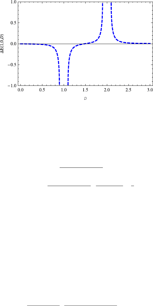
Fig. 13.1 The energy difference E(1, 0,D) decreases with the dimension D ∈ (0, 0.9], while
increases with the dimension D ∈[1.1, 1.9] and then decreases again with the dimension D ≥2.1.
The E(1, 0,D) is symmetric with respect to the point (1.5, 0), so are those E(n, 0,D).The
parameter ξ =0.05 is taken here and also in Figs. 13.2–13.6
For a small ξ ,wehave
E(n,l,D) M
1 −
ξ
2
2[n +(D −3)/2]
2
−
ξ
4
2[n +(D −3)/2]
4
2n +D −3
2l +D −1
−
3
4
, (13.28)
where the first term on the right hand side is the rest energy M (c
2
=1), the second
one is from the solutions of the Schrödinger equation, and the third one is the fine
structure energy, which removes the degeneracy between the states with the same n.
It is found from Eq. (13.28) that the energy levels E(n,l,D) are almost independent
of the quantum number l for a small potential parameter ξ asshowninFig.13.1.
We now determine the normalization factor N
KE
from the normalization condi-
tion
†
KE
KE
dV =1. (13.29)
Since n
=τ −η is a non-negative integer, we may express the confluent hyperge-
ometric functions by the associated Laguerre polynomials (5.21). Through a direct
calculation, we obtain the normalization factor
N
KE
=
(M
2
−E
2
)
1/4
(2η +1)
(τ +η +1)
2Mτ
(K +τ
)(τ −η)!
1/2
. (13.30)

162 13 Dirac Equation with the Coulomb Potential
3 Analysis of the Eigenvalues
We now analyze the properties of eigenvalues. Recently, Nieto has made use of the
concept of the continuous dimension D to study the bound states of quantum system
with a special potential [87]. With this spirit, we attempt to discuss what happened
to a continuous dimension D asshowninRef.[100].
It is shown from Eq. (13.25) that n = 1, 2, 3,... and l = 0, 1,...,n− 1. If the
principal quantum number n and the angular momentum quantum number l are
fixed, the energy difference E(n,l,D) between eigenvalues for dimensions D
and D −1 can be calculated by
E(n,l,D)=E(n,l,D) −E(n,l,D −1)
=M
ξ
|ξ|
1
1 +
ξ
2
(σ +
√
K
2
−ξ
2
)
2
−
1
1 +
ξ
2
(σ +
K
2
1
−ξ
2
)
2
, (13.31)
where
σ =n −l −1,K
1
=(2l +D −2)/2. (13.32)
It is found from Eq. (13.31) that the relation between E(n,l,D)and dimension D
is more complicated than that of the Schrödinger equation case [87]. The problem
arises from the factor
K
2
−ξ
2
(or
K
2
1
−ξ
2
). Therefore, for a weak potential it
is shown from Eqs. (13.2), (13.13) and (13.31) that
D =2(1/2 −l +K)
≥1 +2|ξ |, when l =0 and K>|ξ|,
≤1 −2|ξ |, when l =0 and K<−|ξ|,
(13.33)
and
D =2(1 −l +K)
≥2 +2|ξ |, when l =0 and K
1
> |ξ |,
≤2 −2|ξ |, when l =0 and K
1
< −|ξ |.
(13.34)
We present the variations of energy difference E(n,l,D) on the dimension D
in Figs. 13.1, 13.2, 13.3. We take the parameters M =1 and ξ =0.05 for definite-
ness. It is shown from Fig. 13.1 that there exist two singular points around D ∼ 1
and D ∼ 2forE(1, 0,D). As the dimension D increases, the energy difference
E(1, 0,D) first decreases with the dimension D in the region (0, 0.9] and then
increases with the dimension D in the region [1.1, 1.9], and finally decreases again
with the dimension D ≥ 2.1. In particular, it is found that the energy difference
E(1, 0,D) is symmetric with respect to the point (1.5, 0). The singular points can
be easily explained from Eqs. (13.31), (13.33) and (13.34). That is, notice that there
exist singular points for K
2
=ξ
2
and K
2
1
=ξ
2
. Thus, it is shown from Eqs. (13.33)
and (13.34) that D =1 ±2ξ and D = 2 ±2ξ for l = 0, respectively. It is shown in
Fig. 13.2, where n =2 and l =1, 0, that there are no bound states for D<0.1. This
can also be explained by Eqs. (13.33) and (13.34). As the dimension D increases, the
energy difference E(2, 1,D) monotonically decreases with dimension D ≥ 0.1.
Finally, we show the E(3,l,D) as a function of dimension D in Fig. 13.3, where
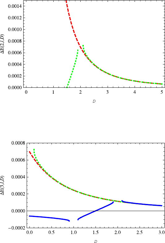
3 Analysis of the Eigenvalues 163
Fig. 13.2 The plot of energy differences E(2,l,D) (l = 0, 1) as a function of dimension D.
Note that E(2, 1,D) decreases with the increasing dimension D ≥0.1 and the variation of the
E(2, 0,D) on the dimension D is very similar to E(1, 0,D)
Fig. 13.3 The plot of energy difference E(3,l,D) as a function of dimension D.Thered
dashed, green dotted and blue solid lines correspond to l =2, 1, 0, respectively
the red dashed, green dotted and blue solid lines correspond to l = 2, 1, 0, respec-
tively. Note that the energy difference E(3, 2,D) decreases monotonically with
the dimension D. The variations of the E(n, 2,D), E(n, 1,D)and E(n, 0,D)
areverysimilartotheE(3, 2,D), E(2, 1,D) and E(1, 0,D), respectively.
Second, we display the variations of energy E(n,l,D) on the dimension D in
Figs. 13.4, 13.5, 13.6. It is shown from Fig. 13.4 that the energy E(1, 0,D) de-
creases with the increasing dimension D ∈ (0, 0.9], but increases with the dimen-
sion D ≥ 1.1. Likewise, this singular point can be explained by Eqs. (13.26)or