Deza M.M., Laurent M. Geometry of Cuts and Metrics
Подождите немного. Документ загружается.

11.1
fl-Embeddings
in
Fixed
Dimension
155
2
4
H
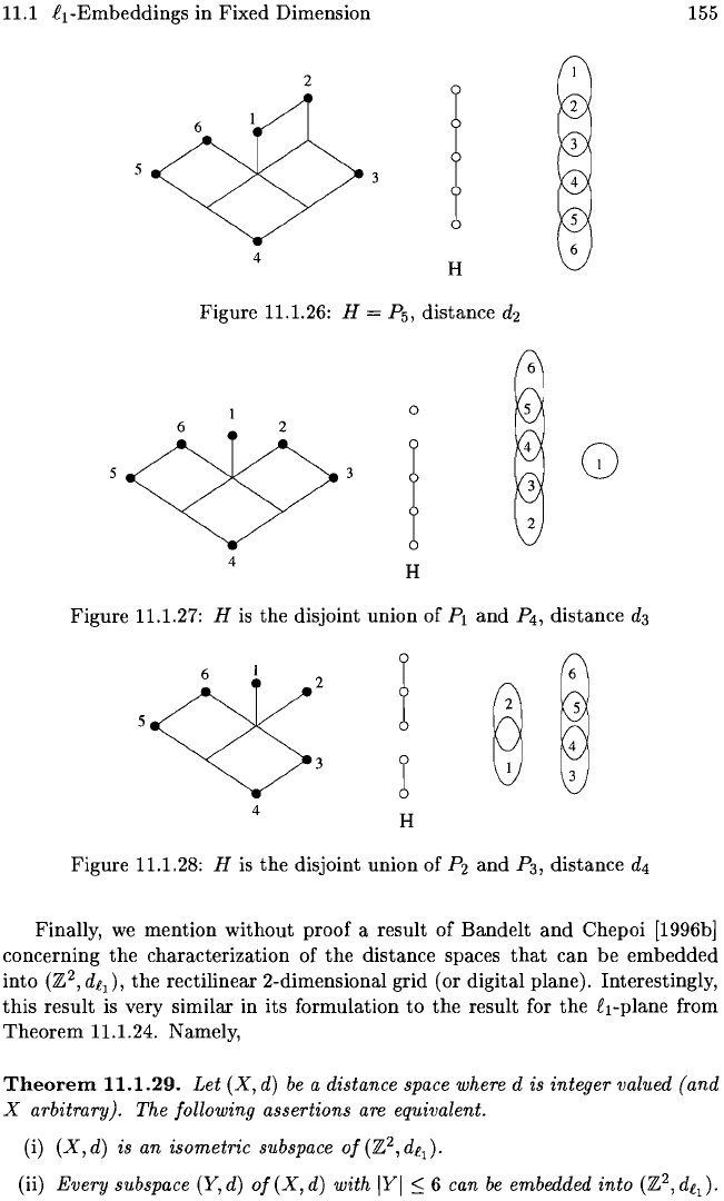
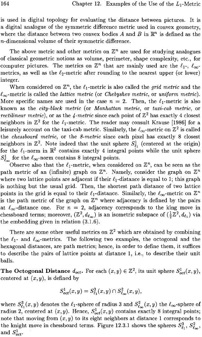
Figure 11.1.26: H = P
5
,
distance d
2
o
2
4
H
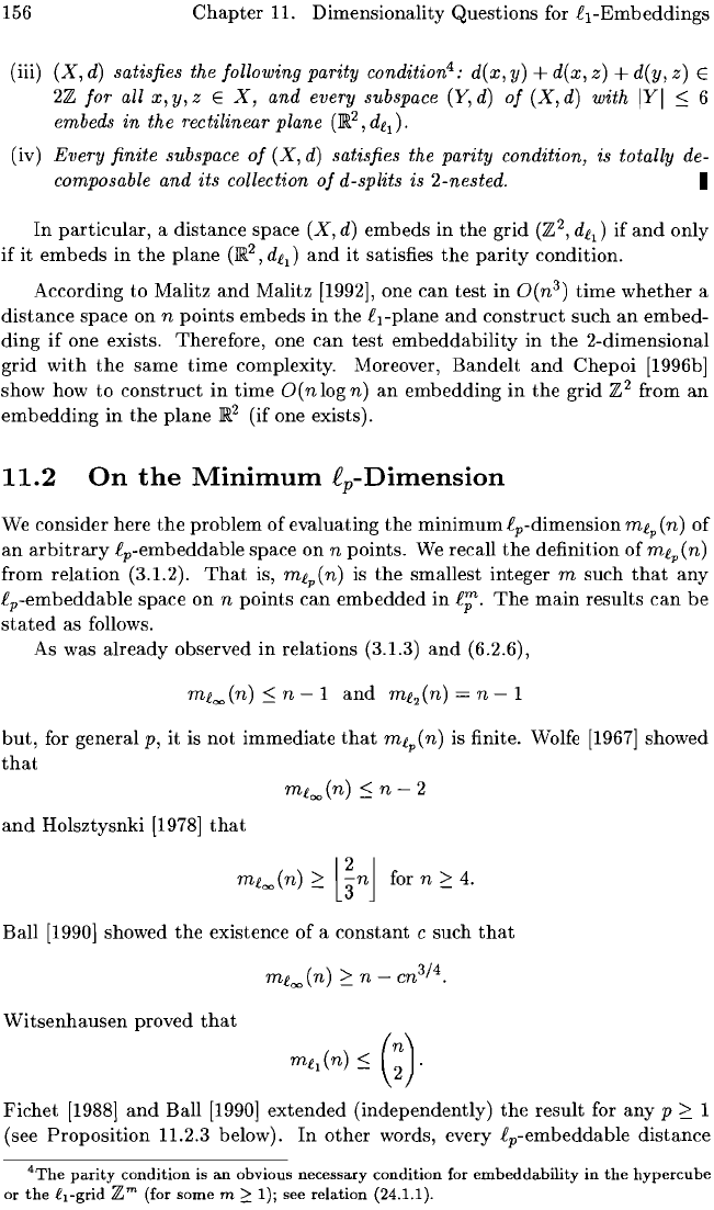
Figure
11.1.27: H
is
the
disjoint union
of
PI
and
P
4
,
distance d
3
2
4
H
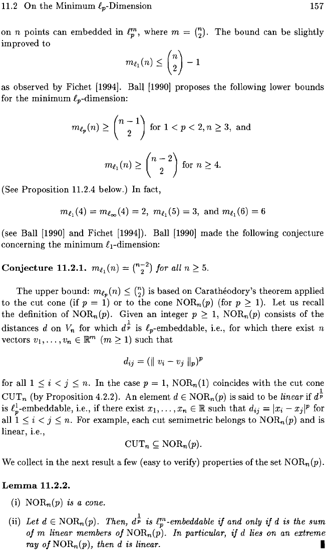
Figure
11.1.28: H
is
the
disjoint union of P
2
and
P
3
,
distance d
4
Finally,
we
mention
without
proof
a result
of
Bandelt
and
Chepoi [1996b]
concerning
the
characterization of
the
distance spaces
that
can
be
embedded
into (Z2,d£1)'
the
rectilinear 2-dimensional grid (or digital plane). Interestingly,
this
result
is very similar in its formulation
to
the
result for
the
£I-plane from
Theorem
11.1.24. Namely,
Theorem
11.1.29.
Let
(X,
d)
be
a distance space where d is
integer
valued
(and
X arbitrary).
The
following
assertions
are equivalent.
(i)
(X,d)
is
an
isometric
subspace
of(Z2,d£1)'
(ii)
Every
subspace
(Y,d)
of
(X,
d)
with
WI:s:
6 can
be
embedded
into
(Z2,d£J.
156
Chapter
11. Dimensionality Questions for fi1-Embeddings
(iii)
(X,
d)
satisfies the following
parity
condition
4
:
d(x,
y) +
d(x,
z)
+
d(y,
z)
E
2/2:
for
all
x,
y,
z E
X,
and
every subspace (Y,
d)
of
(X,
d) with
IYI
:S
6
embeds
in
the rectilinear plane
(~2,
d
fl
).
(iv)
Every
finite
subspace
of
(X,
d)
satisfies the
parity
condition, is totally de-
composable
and
its
collection
of
d-splits is 2-nested. I
In
particular,
a distance space
(X,
d)
embeds in
the
grid
(/2:
2
,
d
fl
) if
and
only
if
it
embeds
in
the
plane
(~2,
d
fl
)
and
it satisfies
the
parity
condition.
According to Malitz
and
Malitz [1992]' one can
test
in
O(n
3
)
time
whether
a
distance
space on n
points
embeds
in
the
fi1-plane
and
construct
such
an
embed-
ding
if
one exists. Therefore, one
can
test
embeddability
in
the
2-dimensional
grid
with
the
same
time
complexity. Moreover,
Bandelt
and
Chepoi [1996b]
show how
to
construct
in
time
0 (n log n)
an
embedding
in
the
grid
/2:
2
from
an
embedding
in
the
plane
~2
(if one exists).
11.2
On
the
Minimum
ep-Dimension
We consider here
the
problem
of
evaluating
the
minimum
fip-dimension
mfp
(n)
of
an
arbitrary
fip-embeddable space
on
n points.
We
recall
the
definition
of
mfp
(n)
from
relation
(3.1.2).
That
is,
mfp(n)
is
the
smallest integer m such
that
any
fip-embeddable space
on
n
points
can
embedded
in
fi;;'.
The
main
results
can
be
stated
as follows.
As was
already
observed
in
relations (3.1.3)
and
(6.2.6),
but,
for general p, it is
not
immediate
that
mfp(n)
is finite. Wolfe
[1967]
showed
that
and
Holsztysnki
[1978]
that
mfoo(n)
2:
l~nJ
for n
2:
4.
Ball
[1990]
showed
the
existence
of
a
constant
c such
that
mfoo(n)
2:
n - cn
3
/
4
•
Witsenhausen
proved
that
mf
l
(n)
:S
(~).
Fichet
[1988]
and
Ball
[1990]
extended
(independently)
the
result for
any
p
2:
1
(see
Proposition
11.2.3 below).
In
other
words, every fip-embeddable
distance
'The
parity
condition
is
an
obvious necessary
condition
for
embeddability
in
the
hypercube
or
the
iI-grid
/2:=
(for
some
m
2:
1); see
relation
(24.1.1).
11.2
On
the
Minimum
Cp-Dimension
157
on
n points
can
embedded
in
C;;',
where m =
G).
The
bound
can be slightly
improved
to
mf,(n)~(;)-1
as observed by Fichet [1994]. Ball
[1990]
proposes the following lower
bounds
for
the
minimum
Cp-dimension:
for
1 < p <
2,
n
~
3,
and
(
n -
2)
mf,(n)
~
2
for n
~
4.
(See
Proposition
11.2.4 below.)
In
fact,
mf,(4)
=
mf=(4)
= 2,
mf,(5)
= 3,
and
mf,(6)
= 6
(see Ball
[1990]
and
Fichet [1994]). Ball
[1990]
made
the
following conjecture
concerning
the
minimum
C I-dimension:
Conjecture
11.2.1.
mf,
(n) =
(n~2)
for
all n
~
5.
The
upper
bound: mfp(n)
~
(~)
is based on
Caratheodory's
theorem applied
to
the
cut
cone (if p =
1)
or to the cone NOR,,(p) (for p
~
1). Let us recall
the
definition
of
NOR,,(p). Given
an
integer p
~
I,
NOR,,(p) consists of
the
,
distances d
on
Vn
for which
d"P
is Cp-embeddable, i.e., for which
there
exist n
vectors
VI,
...
,V
n
E
m.m
(m
~
1) such
that
for all 1
~
i < j
~
n.
In
the
case p =
I,
NOR,,(I) coincides
with
the
cut
cone
1
CUTn
(by
Proposition
4.2.2).
An
element d E NORn(P) is
said
to be
linear
if
d"P
is C!-embeddable, i.e.,
if
there exist Xl,
...
,X
n
E
m.
such
that
dij
=
IXi
-
Xj
IP
for
all
1
~
i < j
~
n. For example, each
cut
semimetric belongs
to
NOR,,(p)
and
is
linear, i.e.,
CUTn
~
NOR,,(p).
We collect
in
the
next result a
few
(easy
to
verify) properties
ofthe
set
NOR"
(p).
LeIllIna
11.2.2.
(i)
NOR,,(p) is a cone.
1
(ii)
Let
d E NOR,,(p).
Then,
d"P
is C;;'-embeddable
if
and
only
if
d is
the
sum
of
m
linear
members
of
NOR,,(p).
In
particular,
if
d lies
on
an
extreme
ray
of
NOR"
(p),
then
d is linear. I
158
Chapter
11. Dimensionality Questions for
fl-Embeddings
Proposition
11.2.3.
mtl
(n)
::;
G)
1
and
mlp(n)
S
G)
for
all p
:2:
1.
Proof. Consider first the case p
1.
We
show
that
every semimetric d E
CUT"
can
be
written
as a nonnegative combination
of
G)
-1
linear
members
of
CUT".
This
follows from
Caratheodory's
theorem
if
d lies
on
the
boundary
of
CUT
n
.
Else,
suppose
that
d lies
in
the interior
of
CUTw
Let a > 0 such
that
d - a6(1)
lies
on
the
boundary
of
CUT".
Then,
d a6(1)
can
be
written
as a nonnegative
combination
of
(~)
1
cut
semimetrics.
This
implies
that
d
can
be
written
as
a nonnegative combination
of
G)
1 linear semimetrics (as 6(1) together
with
any
other
cut
semi metric 6(S) form a nested family).
We
consider now
the
case
p
:2:
1.
Let
H denote
the
hyperplane
in
lIRE",
which is defined by the
equation
L1.~i<j~nXij
=
1.
Set
L;=
{d
E NOR,,(p)
IdE
Hand
d
is
linear}.
One
can
show
that
L is a compact set
and
that
NOR,,(p) n H is a
«(;)
- 1)-
dimensional convex set which coincides with
the
convex hull
of
L. Hence,
Caratheodory's
theorem implies
that
every
member
of
NOR,,(p)
can
be
writ-
ten
as
the
sum
of
G)
linear members
of
NOR,,(p).
This
yields
the
result. I
Proposition
11.2.4.
(i)
ml
l
(n):2:
(n~2)
for
n:2:
4.
(ii)
mtp(n)
:2:
(n~l)
for
1 < p < 2
and
n
:2:
3.
Proof. (i) Set
m:=
C~2).
We
exhibit a semimetric d on
Vn
which
embeds
in
f'{'
but
not
in
if
if
k <
m.
Set d
:=
L 6( {I,
r,
s}); hence,
2~r<s~n-1
for 2
SiS
n
1,
for 2
::;
i < j
::;
n
1,
for 2
::;
i
::;
n
1.
By
construction, d embeds isometrically
in
fr.
We
show
that
d cannot be embed-
ded
in
ff
if
k <
m.
For this,
we
consider
the
inequality
of
negative type (6.1.1)
with
b 1,
...
,1,
-en
-
4»,
i.e., the inequality
(11.2.5)
2(n
4)XIn
2 L
Xli
-
(n
-
4)
L
Xin
+
Xij
S
O.
29~n-1
2~i~n-l
LS':<J:Son--l
Let
F denote
the
face
of
the
cone
NOR,,(l)
(=CUT
n
)
which
is
defined by the
inequality (11.2.5). Clearly,
the
cut
semimetrics
6({1,r,s})
(2
S r < s S n
1)
are
the
only
cut
semimetrics
that
lie on
F.
Moreover,
they
are linearly inde-
pendent.
Hence, F
is
a simplex face
of
NOR,,(l).
Therefore,
dis
fl-rigid;
that
is, d
:=
L 6( {I,
r,
s})
is
its only 114-realization. No two
cut
semimetrics
2<r<s<n-1
6( {I, r,
8})
and
6( {I,
r\
s'})
form a nested pair. Hence,
the
family {6( {I, r,
8})
I
11.2
On
the
Minimum
ip-Dimension
159
2
~
T < S
~
n I} cannot be covered
with
less
than
m
nested
subfamilies.
This
shows
that
d is
not
i~-embeddable
if k <
m.
(ii) We only sketch
the
proof, which is along
the
same lines as for (i). Set
m
(n21).
Consider
the
vectors
VI,
...
,
Vn
E ]Rm defined by
if
T i
if
8 = i
otherwise
for 1
~
T < s <
n.
Define a distance d
on
Vr,
by
setting
~j
Vi
Vj
lip
for
1
~
i < j
~
n.
So d embeds
in
i~
by construction. One
can
show
that
d does
not
embed
in
i;
if
k < m by using, as
in
case (i), a special inequality which is
valid for
the
cone NORn(P)
and
is satisfied
at
equality
by
d
P
•
Namely, one uses
the
inequality:
L
(II
Ui
Uj
IIp)P
(n +
I::;i<j::;n
which holds for any set
of
n vectors
Ul,
.••
,
Un
E
]Rh
(h
~
1)
if
1
~
p
~
2 (Ball
[1987]). I
Remark
11.2.6.
Linial, London
and
Rabinovich
[1994]
define
the
metric
dimension
dim(G)
of
a connected
graph
G as
the
smallest integer m for which
there
exists a norm
II
.
lion
]Rm
such
that
the
graphic space
(V,
d
a
)
of
the
graph
G can be isometrically
embedded
into
the
space
(]Rm,
d!l.II)'
The
definition extends clearly
to
an
arbitrary
semimetric space. Hence,
rather
than
looking only
at
embeddings in a fixed
Banach
ep-space, Linial, London
and
Rabinovich
[1994]
consider embeddings in
an
arbitrary
normed
space.
Actually,
this
notion
of
metric dimension is linked with e(X)-embeddings in
the
fol-
lowing way.
Let
(Vn'
d)
be a semimetric space.
Then,
its metric dimension is equal
to
the
minimum
rank
of
a system
of
vectors
VI,""
Vn
E
]Rk
(k
2:
1)
providing
an
e=-embedding
of
(Vn, d), i.e., such
that
d
ij
=11
Vi
-
Vj
1100
for all 1
:::;
i < j
:::;
n.
The
metric dimension
of
several
graphs
is computed in Linial, London
and
Rabi-
novich [1994]. In
particular,
dim(Kn)
= f1ogz(n)l,
dim(T)
= O(log2(n)) for a tree on
n nodes
(both
being realized by
an
too-embedding),
dim(C
zn
) = n for a circuit on 2n
nodes (realized by
an
tl-embedding),
dim(K
nxz
)
2:
n-l
for
the
cocktail
party
graph.
It
is also shown
there
that,
if G is a
graph
on
n nodes with metric dimension
d,
then
each
vertex
has degree
:::;
3
d
1, G has
diameter
2:
~(n;\
-1),
and
there exists a
subset
S
of
O(dnl-l)
nodes whose deletion disconnects G
and
so
that
each connected component
of
G\S
has no more
than
(1-
~
+
o(l))n
nodes.
Dewdney
[1980]
considers
the
question
of
embedding
graphs
isometrically
into
the
e
p
-
space (Fm, dip), where F is a field. He shows, in particular,
that
every connected
graph
G on n nodes
can
be isometrically embedded
into
the
space
({O,
1, More-
over,
computing
the
smallest m such
that
G embeds isometrically into
({O,
l,2}m,dt=)
is
an
NP-hard
problem. I
M.M. Deza, M. Laurent, Geometry of Cuts and Metrics, Algorithms and Combinatorics 15,
DOI 10.1007/978-3-642-04295-9_12, © Springer-Verlag Berlin Heidelberg 2010
Chapter
12.
Examples
of
the
Use
of
the
L1-Metric
The
L
1
-
metric
is
widely used
in
many
areas, for instance, for
the
analysis
of
data
structures,
for
the
recognition of
computer
pictures, or for comparing
random
variables
in
probabilities. We provide here some (superficial) information on
some areas
of
application
of
the
Lrmetric.
The
importance
of
the
L1-metric is
illustrated,
in
particular,
by
the
great variety of names
under
which it is known.
For example,
the
Manhattan
metric,
the
taxi-cab metric, or
the
4-metric are
different names for
the
same notion, namely,
the
£1
distance
in
the
plane; more
terminology is given
in
Section 12.3.
12.1
The
L1-Metric
in
Probability
Theory
Let
(n,
A,
f.L)
be
a probability space
and
let X : n
-->
~
be
a
random
variable
belonging
to
L
1
(n,
A,
f.L);
that
is, such
that
In
IX(w)If.L(dw)
<
00.
Let
Fx
denote
the
distribution
function
of
X,
Le.,
Fx(x)
=
f.L({w
E n I X(w)
:S
x})
for x E
~
when
it
exists, its derivative
Fx
is
called
the
density
of
X.
A great variety
of
metrics on
random
variables are
studied
in
the
monograph
by Rachev [1991];
among
them,
the
following are based on
the
L
1
-metric:
•
The
usual L1-metric between
the
random
variables:
L1(X,
Y)
=
E(IX
- YI) =
In
IX(w) -
Y(w)If.L(dw).
•
The
Monge-Kantorovich-Wasserstein
metric
(i.e.,
the
L
1
-metric
between
the
distribution
functions):
k(X,
Y)
= k IFx(x) - Fy(x)ldx
•
The
total
valuation metric (i.e.,
the
L
1
-metric between
the
densities when
they
exist):
O"(X,
Y)
=!
r IFx(x) -
F~(x)ldx.
2
JITf.
•
The
engineer metric (Le.,
the
L
1
-metric between
the
expected values):
EN
(X,
Y)
=
IE(X)
- E(Y)I.
162
Chapter
12.
Examples of the Use of
the
L
1
-Metric
•
The
indicator metric:
·i(X,
Y)
=
E(lxfY)
=
11-(
{w
E n I X(w)
=1=
Yew)}).
In
fact, the Lp-analogues
(1
:::;
P
:::;
(0) of
the
above metrics, especially of
the
first two,
are
also used in probability theory.
Several results are known, establishing links among
the
above metrics. One
of
the
main such results is
the
Monge-Kantorovich mass-transportation theorem
which shows
that
the
second metric
k(X,
Y)
can
be
viewed as a minimum
of
the
first metric
L1
(X,
Y)
over all joint distributions of X and Y with fixed marginal.
A relationship between
the
L1(X,
Y)
and the engineer metric
EN
(X,
Y)
is given
in Rachev
[1991]
as a solution
of
a moment problem. Similarly, a connection
between
the
total
valuation metric O'(X,
Y)
and
the
indicator metric
i(X,
Y)
is
given in Dobrushin's theorem on
the
existence and uniqueness
of
Gibbs fields
in
statistical
physics. See Rachev
[1991]
for a detailed account on
the
above topics.
We
mention another example
of
the
use of the L1-metric in probability theory,
namely for Gaussian random fields.
We
refer to Noda [1987,
1989]
for a detailed
account. Let
B =
(B
(x) I x E
M)
be a centered Gaussian system
with
parameter
space
1\1,
0 E
M.
The
variance of the increment is denoted by
d(x,y)
E«B(x)
- B(y))2) for
x,y
EM.
When
(M,
d)
is a metric space which
is
L
1
-embeddable,
the
Gaussian system is
called a Levy's Brownian motion with
parameter
space (AI, d).
The
case M
JllI.n
and
d(x,y)
II
x - y
112
gives
the
usual Brownian motion with n-dimensional parameter. By
Lemma
4.2.5, (AI,
d)
is L1-embeddable if
and
only if there exist a non negative
measure space
(H,
v)
and a mapping x
I->
Ax
~
H with
v(Ax)
<
00
for x E
M,
such
that
d(x,y)
v(Ax6Ay)
for
x,y
E
M.
Hence, a Gaussian system
admits
a representation called
of
Chentsov type
B(x)
= r
W(dh)
for x E M
JAz
in
terms of a Ganssian
random
measure based
on
the
measure space (H, v) with
d(x,
y)
v(Ax6Ay)
if and only
if
dis
Ll-embeddable.
This
Chentsov type representation
can
be
compared
with
the Crofton for-
mula for projective metrics from Theorem 8.3.3. Actually
both
come naturally
together in Ambartzumian
[1982]
(see
parts
A.8-A.9 of Appendix A there).
12.2
The
iI-Metric
in
Statistical
Data
Analysis
A data structure
·is
a pair
(I,
d), where I is a finite set, called population,
and
d : I x I
--+
1I4
is a symmetric mapping with dii 0 for i E
I,
called dissimi-
larity index.
A typical problem in statistical
data
analysis is to choose a "good
12.3
The
f1-Metric
in
Computer
Vision
and
Pattern
Recognition
163
representation"
of
a
data
structure;
usually, "good"
means
a
representation
al-
lowing
to
represent
the
data
structure
visually by a graphic display. Each
sort
of
visual display corresponds,
in
fact,
to
a special choice
of
the
dissimilarity index
as a distance
and
the
problem
turns
out
to
be
the
classical isometric
embedding
problem
in special classes
of
metrics.
For instance, in hierarchical classification,
the
case
when
d is
ultrametric
corresponds
to
the
possibility
of
having a representation
of
the
data
structure
by a so-called indexed hierarchy (see
Johnson
[1967]). A
natural
extension
is
the
case
when
d is
the
path
metric
of
a weighted tree, i.e.,
when
d satisfies
the
four
point
condition
(cf.
Section 20.4);
then
the
data
structure
is
called
an
additive
tree.
Data
structures
(J,
d)
for which d is f
2
-embeddable are considered
in
factor
analysis
and
multidimensional scaling. These two cases
together
with
cluster
analysis are
the
main
three
techniques for
studying
data
structures.
The
case
when
d is f1-embeddable is a
natural
extension
of
the
ultrametric
and
f2
cases
which
has
received considerable
attention
in
the
recent years.
An
fp-approximation consists
of
minimizing
the
estimator
II
e
lip,
where e
is a vector or a
random
variable (representing
an
error, deviation, etc).
The
following
criteria
are used
in
statistical
data
analysis:
•
the
f
2
-norm,
in
the
least square
method;
or
its square,
•
the
foo-norm,
in
the
minimax
method,
•
the
f1-norm,
in
the
least absolute values (LAV)
method.
In
fact,
the
f1
criterion has also been increasingly used
in
the
recent years.
The
importance
ofthe
role played by
the
f1-metric in
statistical
data
analysis
can
be seen, for instance, from
the
volumes by Dodge [1987b, 1992]
and
by
van
Cutsem
[1994]
of
proceedings
of
conferences
on
the
topic
of
statistical
data
analysis. We refer, in
particular,
to
the
papers
by Crichtley
and
Fichet
[1994]'
Dodge [1987a],
Fichet
[1987a, 1987b, 1992, 1994], Le Calve [1987],
Vajda
[1987]
in
those
volumes.
12.3
The
.e1-Metric
in
Computer
Vision
and
Pattern
Recognition
The
fp-metrics are also used in
the
new
area
called
pattern
recognition, or
robot
vision,
or
digital
topology; see, e.g., Rosenfeld
and
Kak
[1976],
Horn
[1986].
A
computer
picture
is a
subset
of
zn
(or
of
a scaling
~zn
of
zn)
which is
called a
digital
n-D-space
(or
an
n-D
m-quantized
space). Usually,
pictures
are
represented
in
the
digital plane
Z2
or
in
the
digital 3-D-space Z3.
The
points
of
zn
are called
the
pixels.
Given a
picture
in
zn,
i.e., a subset A
of
zn,
one way
to
define
its
volume
vol(A) is by vol(A)
:=
IAI,
i.e., as
the
number
of
pixels contained in A.
Then,
the
distance
d(A,
B)
:=
vol(A6.B)
164
Chapter
12.
Examples
of
the
Use
of
the
L1-Metric
is used
in
digital
topology for evaluating
the
distance
between pictures.
It
is
a
digital
analogue
of
the
symmetric
difference
metric
used
in
convex geometry,
where
the
distance
between two convex bodies A
and
B
in
ffi.n
is defined as
the
n-dimensional
volume
of
their
symmetric
difference.
The
above
metric
and
other
metrics
on
zn
are
used for
studying
analogues
of
classical geometric notions as volume,
perimeter,
shape
complexity, etc., for
computer
pictures.
The
metrics
on
zn
that
are
mainly
used
are
the
fi
1
-,
fi
oo
-
metrics,
as well as
the
fi
2
-metric
after
rounding
to
the
nearest
upper
(or lower)
integer.
When
considered
on
zn,
the
fi
1
-metric
is also called
the
grid metric
and
the
fioo-metric is called
the
lattice metric (or Chebyshev metric, or uniform metric).
More
specific
names
are
used
in
the
case n =
2.
Then,
the
fi
1
-metric
is also
known
as
the
city-block metric (or Manhattan metric, or taxi-cab metric, or
rectilinear metric), or as
the
4-metric since each
point
of
Z2 has exactly 4 closest
neighbors
in
Z2 for
the
fi
1
-metric.
The
reader
may
consult
Krause
[1986] for a
leisurely account
on
the
taxi-cab
metric. Similarly,
the
fioo-metric
on
Z2 is called
the
chessboard metric, or
the
8-metric since each pixel has
exactly
8 closest
neighbors
in
Z2. Note indeed
that
the
unit
sphere
Sl,
(centered
at
the
origin)
for
the
fi
1
-norm
in
ffi.2 contains exactly 4
integral
points
while
the
unit
sphere
SL
for
the
fioo-norm contains 8
integral
points.
Observe also
that
the
fi
1
-metric,
when
considered
on
zn,
can
be
seen as
the
path
metric
of
an
(infinite)
graph
on
zn.
Namely, consider
the
graph
on
zn
where two
lattice
points
are
adjacent
if
their
fi
1
-distance is equal
to
1;
this
graph
is
nothing
but
the
usual
grid.
Then,
the
shortest
path
distance
of
two
lattice
points
in
the
grid
is equal
to
their
fi
1
-distance. Similarly,
the
fioo-metric
on
zn
is
the
path
metric
of
the
graph
on
zn
where adjacency is defined by
the
pairs
at
fioo-distance one. For n =
2,
adjacency corresponds
to
the
king move
in
chessboard
terms; moreover, (Z2, d
too
) is
an
isometric subspace of
(~Z2,
d
t
,)
via
the
embedding
given
in
relation
(3.1.6).
There
are
some
other
useful
metrics
on
Z2 which are
obtained
by combining
the
fi
1
-
and
fioo-metrics.
The
following two examples,
the
octogonal
and
the
hexagonal
distances, are
path
metrics; hence,
in
order
to
define
them,
it
suffices
to
describe
the
pairs
of
lattice
points
at
distance
1,
i.e.,
to
describe
their
unit
balls.
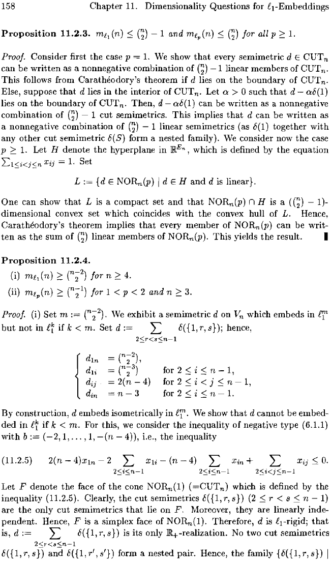
The
Octogonal
Distance
doct.
For each (x, y) E
Z2,
its
unit
sphere
S;ct(x, y),
centered
at
(x, y), is defined by
S;ct(x, y) =
si,
(x, y) n
SL(x,
y),
where
Si,(x,y)
denotes
the
fi
1
-sphere of
radius
3
and
SL(x,y)
the
fioo-sphere
of
radius
2,
centered
at
(x, y). Hence, S;ct(x, y) contains exactly 8
integral
points;
note
that
moving from (x, y)
to
its
eight neighbors
at
distance
1 corresponds
to
the
knight
move
in
chessboard
terms.
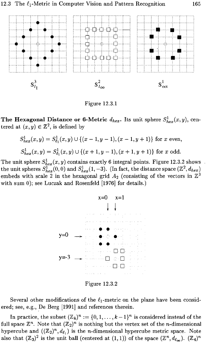
Figure
12.3.1 shows
the
spheres Si"
SL,
and
S~ct.
12.3
The
£l-Metric
in
Computer
Vision
and
Pattern
Recognition
: :
······nnnnn~·
:L
.....•
•
•.
, e
H
'
••
•
.~
'l
..........
.
• •
e :
••
•
...
.
"
..•
:
; .
. .
•...........••...•
'
H"""'"H'"'",,,,'
Figure
12.3.1
.H·
•
• •
iii'
165
The
Hexagonal
Distance
or
6-Metric
dhexo
Its
unit sphere Skex(x, y), cen-
tered
at
(x,
y)
E Z2, is defined by
Skex(x,
y)
= s1
1
(x,
y)
U
{(x
-
1,
y - 1), (x - 1, y +
I)}
for x even,
Skex(x,
y)
= s1
1
(x,
y)
U
{(x
+ 1, y - 1), (x + 1, y +
I)}
for x odd.
The
unit
sphere
Skex(x,
y)
contains exactly 6 integral points.
Figure
12.3.2 shows
the
unit
spheres
Skex(O,
0)
and
Skex(l,
-3).
(In
fact,
the
distance
space (Z2, d
hex
)
embeds
with
scale 2
in
the
hexagonal grid
A2
(consisting
of
the
vectors
in
Z3
with
sum
0); see Luczak
and
Rosenfeld
[1976]
for details.)
y=o _
y=-3
----.
x=O
x=l
• •
•
• •
o
•
00
o
DO
Figure 12.3.2
Several
other
modifications
of
the
£l-metric on
the
plane have
been
consid-
ered; see, e.g.,
De
Berg
[1991]
and
references therein.
In
practice,
the
subset
(Zk)n
:=
{O,
1,
...
,k
_l}n
is considered
instead
of
the
full space
zn.
Note
that
(Z2)n is nothing
but
the
vertex set
of
the
n-dimensional
hypercube
and
((Z2)n,dl
1
)
is
the
n-dimensional hypercube
metric
space.
Note
also
that
(Z3)2
is
the
unit
ball
(centered
at
(1,1))
of
the
space
(zn,
d
loo
)' (Z4)n