Cold and Hot Forging: Fundamentals and Applications / Edited by Taylan Altan, Gracious Ngaile, Gangshu Shen

Подождите немного. Документ загружается.

98 / Cold and Hot Forging: Fundamentals and Applications

on both the top and bottom surfaces of the de-

forming part. Thus,

V4ps V

DiD

E ⳱ 2 s r2prdr ⳱ rdr

冮冮

2h 2h

or, with s ⳱ m¯r/3,

冪

2¯r V

E ⳱ pm R (Eq 9.27)

冪

The total energy rate is:

˙˙˙

E ⳱ E Ⳮ E

TDF

2¯r V

E ⳱ pR¯rV Ⳮ pm R (Eq 9.28)

冪

The load is:

E2R

L ⳱⳱pR¯r 1 Ⳮ m (Eq 9.29)

冢冣

冪

Comparison of Eq 9.29 and 9.24 indicates that

in axisymmetric homogeneous upsetting the

loads calculated by the slab and upper-bound

methods both give the same end result.

9.3.3 Application to

Nonhomogeneous Upsetting

Homogeneous upsetting can only be achieved

at low strains and with nearly perfect lubrica-

tion. In all practical upsetting operations, the

friction at the die/material interface prevents the

metal from ﬂowing radially in a uniform fash-

ion. As a result, bulging of the free surfaces oc-

curs, and the radial and axial velocities are func-

tions of z as well as of r. In this case, a velocity

ﬁeld may be given by [Lee et al., 1972]:

v ⳱ 0 (Eq 9.30a)

v ⳱ⳮ2Az(1 ⳮ bz /3) (Eq 9.30b)

v ⳱ A(1 ⳮ bz )r (Eq 9.30c)

where b is a parameter representing the severity

of the bulge, and A is determined from the ve-

locity boundary condition at z ⳱ h, to be:

A ⳱

2h(1 ⳮ bh /3)

The strain rates are:

˙e ⳱⳱A(1 ⳮ bz ) (Eq 9.31a)

˙e ⳱⳱A(1 ⳮ bz ) (Eq 9.31b)

˙e ⳱⳱ⳮ2A(1 ⳮ bz ) (Eq 9.31c)

˙c ⳱ ˙c ⳱ 0;

rhhz

⳵v ⳵v

˙c ⳱Ⳮ ⳱ⳮ2Abzr (Eq 9.31d)

⳵z ⳵r

The effective strain rate is calculated from:

1/2

222 2

¯e ⳱ ˙e Ⳮ ˙e Ⳮ ˙e Ⳮ ˙c

r h zrz

冤冢冣冥

22 21/2

¯e ⳱ [3(1 ⳮ bz) Ⳮ (brz) ] (Eq 9.32)

冪

The total energy dissipation, E

, given by Eq

9.25 can now be calculated analytically or nu-

merically. The exact value of b is determined

from the minimization condition, i.e., from:

⳵E

⳱ 0

⳵b

The value of b, obtained from Eq 9.33, is used

to calculate the velocities and strain rates that

then give the minimum value of the energy rate,

min

. The upsetting load is then given by:

L ⳱ E/V

min D

9.4 Finite Element

Method in Metal Forming

The basic approach of the ﬁnite element (FE)

method is one of discretization. The FE model

is constructed in the following manner [Kobay-

ashi et al., 1989]:

●

A number of ﬁnite points are identiﬁed in

the domain of the function and the values of

Methods of Analysis for Forging Operations / 99

the function and its derivatives, when appro-

priate, are speciﬁed at these points.

●

The domain of the function is represented

approximately by a ﬁnite collection of sub-

domains called ﬁnite elements.

●

The domain is then an assemblage of ele-

ments connected together appropriately on

their boundaries.

●

The function is approximated locally within

each element by continuous functions that

are uniquely described in terms of the nodal

point values associated with the particular

element.

The path to the solution of a ﬁnite element

problem consists of ﬁve speciﬁc steps: (1) iden-

tiﬁcation of the problem, (2) deﬁnition of the

element, (3) establishment of the element equa-

tion, (4) the assemblage of element equations,

and (5) the numerical solution of the global

equations. The formation of element equations

is accomplished from one of four directions: (a)

direct approach, (b) variational method, (c)

method of weighted residuals, and (d) energy

balance approach.

The main advantages of the FE method are:

●

The capability of obtaining detailed solu-

tions of the mechanics in a deforming body,

namely, velocities, shapes, strains, stresses,

temperatures, or contact pressure distribu-

tions

●

The fact that a computer code, once written,

can be used for a large variety of problems

by simply changing the input data

9.4.1 Basis for the

Finite Element Formulation

The basis for the ﬁnite element metal forming

formulation, using the “variational approach,” is

to formulate the proper functional (function of

functions) depending on speciﬁc constitutive re-

lations. The variational approach is based on one

of two variational principles. It requires that

among admissible velocities u

that satisfy the

conditions of compatibility and incompressibil-

ity, as well as the velocity boundary conditions,

the actual solution gives the following func-

tional a stationary value [Kobayashi et al.,

1989]:

p ⳱ ¯r ¯edV ⳮ F u dS (Eq 9.35a)

冮冮

(for rigid-plastic materials) and:

p ⳱ E(˙e )dV ⳮ F u dS (Eq 9.35b)

ij i i

冮冮

(for rigid-viscoplastic materials) where is the¯r

effective stress, is the effective strain rate, F

¯e

represents surface tractions, is the workE(˙e )

function, and V and S the volume and surface

of the deforming workpiece, respectively. The

solution of the original boundary-value problem

is then obtained from the solution of the dual-

variational problem, where the ﬁrst-order vari-

ation of the functional vanishes, namely:

dp ⳱ ¯rd ¯edV ⳮ F dudS⳱ 0 (Eq 9.36)

冮冮

where for the rigid-

¯r ⳱ ¯r(¯e) and ¯r ⳱ ¯r(¯e,¯e)

plastic and rigid-viscoplastic materials, respec-

tively.

For an accurate ﬁnite element prediction of

material ﬂow in a forging process, the formula-

tion must take into account the large plastic de-

formation, incompressibility, workpiece-tool

contact, and, when necessary, temperature cou-

pling.

The basic equations to be satisﬁed are the

equilibrium equation, the incompressibility con-

dition, and the constitutive relationship. When

applying the penalty method, the velocity is the

primary solution variable. The variational equa-

tion is in the form [Li et al., 2001]:

dp(v) ⳱ ¯rd¯edV Ⳮ K˙ed˙e dV

冮冮

ⳮ F dudS ⳱ 0 (Eq 9.37)

冮

where K, a penalty constant, is a very large posi-

tive constant.

An alternative method of removing the in-

compressibility constraint is to use a Lagrange

multiplier [Washizu, 1968] and [Lee et al., 1973]

and modifying the functional by adding the term

is the volumetric兰k˙e dV, where ˙e ⳱ ˙e ,

vvii

strain rate. Then:

dp ⳱ ¯rd ¯edV Ⳮ kd˙e dV

冮冮

Ⳮ ˙edkdV ⳮ F dudS⳱ 0 (Eq 9.38)

冮冮

In the mixed formulation, both the velocity

and pressure are solution variables. They are

100 / Cold and Hot Forging: Fundamentals and Applications

solved by the following variational equation [Li

et al., 2001],

dp(v,p) ⳱ ¯rd ¯edV Ⳮ pd ˙e dV Ⳮ ˙edp

冮冮冮

VV V

ⳮ F dudS ⳱ 0 (Eq 9.39)

冮

where p is the pressure.

Equations 9.37 to 9.39 can be converted into

a set of algebraic equations by utilizing the stan-

dard FEM discretization procedures. Due to the

nonlinearity involved in the material properties

and frictional contact conditions, this solution is

obtained iteratively.

The temperature distribution of the workpiece

and/or dies can be obtained readily by solving

the energy balance equation rewritten by using

the weighted residual method as [Li et al., 2001]:

kT dTdVⳭ qcTdTdV

ij ij

冮冮

ⳮ ␣ ¯r ¯edTdV ⳱ q dTdS (Eq 9.40)

冮冮

where k is the thermal conductivity, T the tem-

perature, q the density, c the speciﬁc heat, ␣ a

fraction of deformation energy that converts into

heat, and q

the heat ﬂux normal to the boundary,

including heat loss to the environment and fric-

tion heat between two contacting objects. Using

FEM discretization, Eq 9.40 can also be con-

verted to a system of algebraic equations and

solved by a standard method. In practice, the

solutions of mechanical and thermal problems

are coupled in a staggered manner. After the

nodal velocities are solved at a given step, the

deformed conﬁguration can be obtained by up-

dating the nodal coordinates [Li et al., 2001].

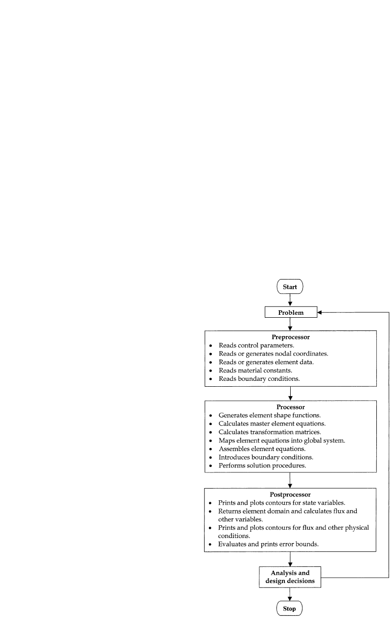
9.4.2 Computer Implementation of the

Finite Element Method

Computer implementation of the basic steps

in a standard ﬁnite element analysis consists of

three distinct units, viz. the preprocessor, pro-

cessor, and the postprocessor.

Preprocessor. This operation precedes the

analysis operation. It takes in minimal infor-

mation from the user (input) to generate all nec-

essary problem parameters (output) required for

a ﬁnite element analysis.

The input to the preprocessor includes infor-

mation on the solid model, discretization re-

quirements, material identiﬁcation and parame-

ters, and boundary conditions; whereas the

output includes coordinates for nodes, element

connectivity and element information, values of

material parameters for each element, and

boundary loading conditions on each node.

In the preprocessing stage, a continuum is di-

vided into a ﬁnite number of subregions (or ele-

ments) of simple geometry (triangles, rectan-

gles, tetrahedral, etc.). Key points are then

selected on elements to serve as nodes where

problem equations such as equilibrium and com-

patibility are satisﬁed.

In general, preprocessing involves the follow-

ing steps to run a successful simulation using a

commercial FE package:

1. Select the appropriate geometry/section for

simulation based on the symmetry of the

component to be analyzed.

2. Assign workpiece material properties in the

form of the ﬂow stress curves. These may be

user deﬁned or selected from the database

provided in the FE package.

3. Mesh the workpiece using mesh density win-

dows, if necessary, to reﬁne mesh in critical

areas.

4. Deﬁne the boundary conditions (velocity,

pressure, force, etc.). Specify the movement

and direction for the dies. Specify the inter-

face boundary and friction conditions. This

prevents penetration of the dies into the

workpiece and also affects the metal ﬂow de-

pending on the friction speciﬁed. In massive

forming processes such as forging, extrusion,

etc., the shear friction factor “m” is speciﬁed.

Note: If die stress analysis or thermal analysis

is required, one would need to mesh the dies and

specify the material properties for them. Also

die and workpiece temperatures and interface

heat transfer coefﬁcients would need to be spec-

iﬁed. Material data at elevated temperatures

would be required for the tools and the work-

piece. The die stress analysis procedure is de-

scribed in Chapter 16 on process modeling in

impression die forging.

Processor. This is the main operation in the

analysis. The output from the preprocessor (in-

cluding nodal coordinates, element connectivity,

material parameters, and boundary/loading con-

ditions) serves as the input to this module. It

establishes a set of algebraic equations that are

to be solved, from the governing equations of

the boundary value problem. The governing

Methods of Analysis for Forging Operations / 101

Fig. 9.4 Flowchart of ﬁnite element implementation

equations include conservation principles, ki-

nematic relations, and constitutive relations. The

FE engine/solver then solves the set of linear or

nonlinear algebraic equations to obtain the state

variables at the nodes. It also evaluates the ﬂux

quantities inside each element.

The following steps are pursued in this opera-

tion:

1. A suitable interpolation function is assumed

for each of the dependent variables in terms

of the nodal values.

2. Kinematic and constitutive relations are sat-

isﬁed within each element.

3. Using work or energy principles, stiffness

matrices and equivalent nodal loads are es-

tablished.

4. Equations are solved for nodal values of the

dependent variables.

Postprocessor. This operation prints and

plots the values of state variables and ﬂuxes in

the meshed domain. Reactions may be evalu-

ated. Output may be in the form of data tables

or as contour plots.

Figure 9.4 shows a ﬂowchart, which shows

the sequence of ﬁnite element implementation

in analysis of metal forming processes.

In interpreting FE results, careful attention is

required since the idealization of the physical

problem to a mathematical one involves certain

assumptions that lead to the differential equation

governing the mathematical model. As illus-

trated in Fig. 9.5, reﬁnement of the mesh size,

alteration of the boundary conditions, etc., may

be needed to increase the accuracy of the solu-

tion.

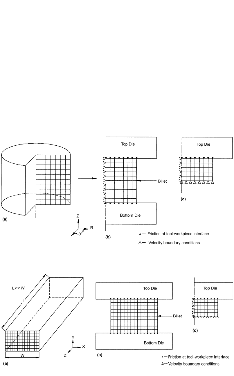
9.4.3 Analysis of Axisymmetric

Upsetting by the FE Method

The use of the FE method in analysis of forg-

ing processes is discussed with the help of a sim-

ple cylindrical compression simulation. Figure

9.6(a) shows the cutaway of a cylinder, which is

to be upset. Since the cylinder is symmetric

about the central axis, i.e., axisymmetric, a 2-D

simulation is adequate to analyze the metal ﬂow

during deformation. Figure 9.6(b) shows the half

model selected for simulation as a result of ro-

tational symmetry, with the nodes along the axis

of symmetry (centerline) restricted along the R-

direction. This model can be further simpliﬁed

to yield a quarter model (Fig. 9.6c) with veloc-

ity/displacement boundary conditions restricting

the movement of the nodes along the Z-direction

as shown. The boundary conditions necessary to

be prescribed for this problem under isothermal

conditions can be summarized as:

●

Velocity/displacement boundary conditions

depending on the symmetry of the work-

piece, to restrict to movement of nodes along

the planes of symmetry as required

●

Die movement and direction according to the

process being analyzed

●

Interface friction conditions at the surfaces

of contact between the tools and the work-

piece

9.4.4 Analysis of

Plane Strain Deformation

Figure 9.7 shows the setup of an FE model

for a plane strain condition. In this case the part

has a uniform cross section along the length and

102 / Cold and Hot Forging: Fundamentals and Applications

Fig. 9.5 The process of ﬁnite element analysis. [Bathe, 1996]

the strain along the Z or length direction is neg-

ligible; i.e., e

is negligible. Hence, only the two-

dimensional cross section shown in Fig. 9.7(b)

is selected for process simulation.

The procedure for simulation is the same as

mentioned for the axisymmetric case. However,

the velocity boundary conditions are different

since the metal is free to ﬂow in the X direction

(Fig. 9.7b). If, however, the cross section is uni-

form, a quarter model can be used for simulation

as shown in Fig. 9.7(c) with velocity boundary

conditions similar to those used for the axisym-

metric case discussed in the previous section. It

should be noted, however, that the results ob-

tained from the plane strain simulation have to

be multiplied by the length of the billet used for

the forging process to get the ﬁnal results.

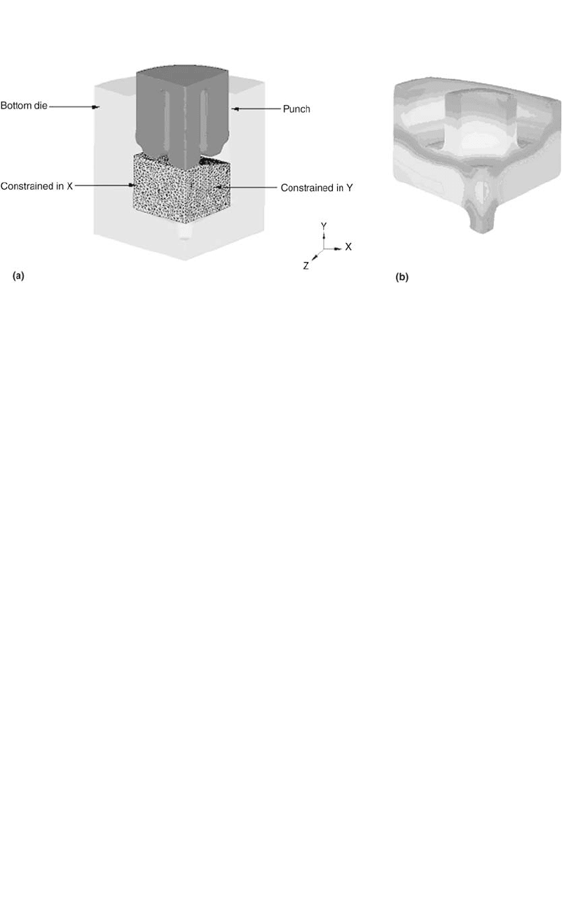
9.4.5 Three-Dimensional

Nonisothermal FE Analysis

Figure 9.8 shows the FE model of the hot

forging process of an automotive component.

The starting preform geometry is not axisym-

metric; hence a 2-D simulation could not be used

to analyze the metal ﬂow. The preform is, how-

ever, symmetric, and hence a quarter model

could be used for modeling the process. Since

the forging process is performed at elevated tem-

peratures, a nonisothermal simulation is con-

ducted. The simulation input differs from those

of an isothermal simulation in the following

ways:

●

Tool and workpiece temperatures have to be

considered, and thermal properties such as

Methods of Analysis for Forging Operations / 103

Fig. 9.7 Analysis of plane strain upsetting by the FE method. (a) Part for plane strain upsetting. (b) Full model. (c) Quarter model

Fig. 9.6

Analysis of axisymmetric cylinder upsetting using the FE method. (a) Cutaway of the cylinder. (b) Half model. (c) Quarter

model

thermal conductivity, heat capacity, interface

heat transfer coefﬁcients, etc. have to be

speciﬁed.

●

Die and workpiece material properties are

speciﬁed as a function of temperature and

strain rate. Dies (still considered as rigid)

have to be meshed since heat transfer be-

tween workpiece and tools is simulated.

The boundary conditions in a 3-D simulation are

similar to those in a 2-D process:

●

Velocity/displacement boundary conditions

need to be speciﬁed depending on the work-

piece geometry. In Fig. 9.8(b), movement of

the boundary nodes is restricted along the

planes of symmetry.

●

Interface friction is speciﬁed depending on

the type of lubrication at the tool/workpiece

interface. In addition to the friction, the in-

terface heat transfer coefﬁcient is also a criti-

cal input to the simulation.

9.4.6 Mesh Generation in FE

Simulation of Forging Processes

Bulk forming processes are generally char-

acterized by large plastic deformation of the

104 / Cold and Hot Forging: Fundamentals and Applications

Fig. 9.8 Three-dimensional non-isothermal FE simulation of a forging process. (a) FE model. (b) Final part with temperature contour.

workpiece accompanied by signiﬁcant relative

motion between the deforming material and the

tool surfaces. The starting mesh in the FE simu-

lation is generally well deﬁned with the help of

mesh density windows to reﬁne the mesh in

critical areas. However, as the simulation pro-

gresses the mesh tends to get signiﬁcantly dis-

torted. This calls for (a) the generation of a new

mesh taking into consideration the updated ge-

ometry of the workpiece and (b) interpolation of

the deformation history from the old mesh to the

new mesh. Current commercial FE codes, such

as DEFORM娂 accomplish this using automatic

mesh generation (AMG) subroutines. AMG ba-

sically determines the optimal mesh density dis-

tribution and generates the mesh based on the

given density. Once the mesh density was de-

ﬁned, the mesh generation procedure considers

the following factors [Altan et al., 1979]:

●

Geometry representation.

●

Density representation. The density speciﬁ-

cation is accommodated in the geometry.

●

Identiﬁcation of critical points (like sharp

corner points) for accurate representation of

the geometry.

●

Node generation. The number of nodes be-

tween critical points are generated and re-

positioned based on the density distribution.

●

Shape improvement and bandwidth mini-

mization. The shape of the elements after the

mesh generation procedure has to be

smoothed to yield a usable mesh. Also the

bandwidth of the stiffness matrix has to be

improved to obtain a computationally efﬁ-

cient mesh.

The FE modeling inputs and outputs are dis-

cussed in detail in Chapter 16 on process mod-

eling.

FE simulation is widely used in the industry

for the design of forging sequences, prediction

of defects, optimization of ﬂash dimensions, die

stress analysis, etc. A number of commercial FE

codes are available in the market for simulation

of bulk forming processes, viz. DEFORM娂,

FORGE娂, QFORM娂, etc. Some practical ap-

plications of FE simulation in hot and cold forg-

ing processes are presented in Chapters 16 and

18.

REFERENCES

[Altan et al., 1979]: Altan, T., Lahoti, G.D.,

“Limitations, Applicability and Usefulness of

Different Methods in Analyzing Forming

Problems,” Ann. CIRP, Vol 28 (No. 2), 1979,

p 473.

[Avitzur, 1968]: Avitzur, B., Metal Forming:

Processes and Analysis, McGraw-Hill,

1968.

[Bathe, 1996]: Bathe, K.J., Finite Element Pro-

cedures, Prentice Hall, 1996.

[Becker, 1992]: Becker, A.A., The Boundary

Element Method in Engineering, McGraw-

Hill International Editions, 1992.

[Hoffman et al., 1953]: Hoffman, O., Sachs, G.,

Introduction to the Theory of Plasticity for

Engineers, McGraw-Hill, 1953.

[Kobayashi et al., 1989]: Kobayashi, S., Oh,

S.I., Altan, T., Metal Forming and the Finite

Element Method, Oxford University Press,

1989.

Methods of Analysis for Forging Operations / 105

[Lee et al., 1972]: Lee, C.H., Altan, T., “Inﬂu-

ence of Flow Stress and Friction upon Metal

Flow in Upset Forging of Rings and Cylin-

ders,” ASME Trans., J. Eng. Ind., Aug 1972,

p 775.

[Lee et al., 1973]: Lee, C.H., Kobayashi, S.,

“New Solutions to Rigid-Plastic Deformation

Problems using a Matrix Method,” Trans.

ASME, J. Eng. Ind., Vol 95, p 865.

[Li et al., 2001]: Li, G., Jinn, J.T., Wu, W.T.,

Oh, S.I., “Recent Development and Applica-

tions of Three-Dimensional Finite Element

Modeling in Bulk Forming Processes,” J. Ma-

ter. Process. Technol., Vol 113, 2001, p 40–

45.

[Thomsen et al., 1954]: Thomsen, E.G., Yang,

C.T., Bierbower, J.B., “An Experimental In-

vestigation of the Mechanics of Plastic De-

formation of Metals,” Univ. of California

Pub. Eng., Vol 5, 1954.

[Thomsen et al., 1965]: Thomsen, E.G., Yang,

C.T., Kobayashi, S., Mechanics of Plastic De-

formation in Metal Processing, Macmillan,

1965.

[Washizu, 1968]: Washizu, K., Variational

Methods in Elasticity and Plasticity, Perga-

mon Press, Oxford, 1968.

SELECTED REFERENCE

[Altan et al., 1983]: Altan, T., Oh, S.I., Gegel,

H., Metal Forming: Fundamentals and Appli-

cations, ASM International, 1983.

CHAPTER 10

Principles of Forging Machines

Manas Shirgaokar

10.1 Introduction

In a practical sense, each forming process is

associated with at least one type of forming ma-

chine (or “equipment,” as it is sometimes called

in practice). The forming machines vary in fac-

tors such as the rate at which energy is applied

to the workpiece and the capability to control

the energy. Each type has distinct advantages

and disadvantages, depending on the number of

forgings to be produced, dimensional precision,

and the alloy being forged. The introduction of

a new process invariably depends on the cost

effectiveness and production rate of the machine

associated with that process. Therefore, capabil-

ities of the machine associated with the new pro-

cess are of paramount consideration. The form-

ing (industrial, mechanical, or metallurgical)

engineer must have speciﬁc knowledge of form-

ing machines so that he/she can:

●

Use existing machinery more efﬁciently

●

Deﬁne with accuracy the existing plant ca-

pacity

●

Better communicate with, and at times re-

quest improved performance from, the ma-

chine builder

●

If necessary, develop in-house proprietary

machines and processes not available in the

machine-tool market

10.2 Interaction between

Process Requirements and

Forming Machines

The behavior and characteristics of the form-

ing machine inﬂuence:

●

The ﬂow stress and workability of the de-

forming material

●

The temperatures in the material and in the

tools, especially in hot forming

●

The load and energy requirements for a

given product geometry and material

●

The “as-formed” tolerances of the parts

●

The production rate

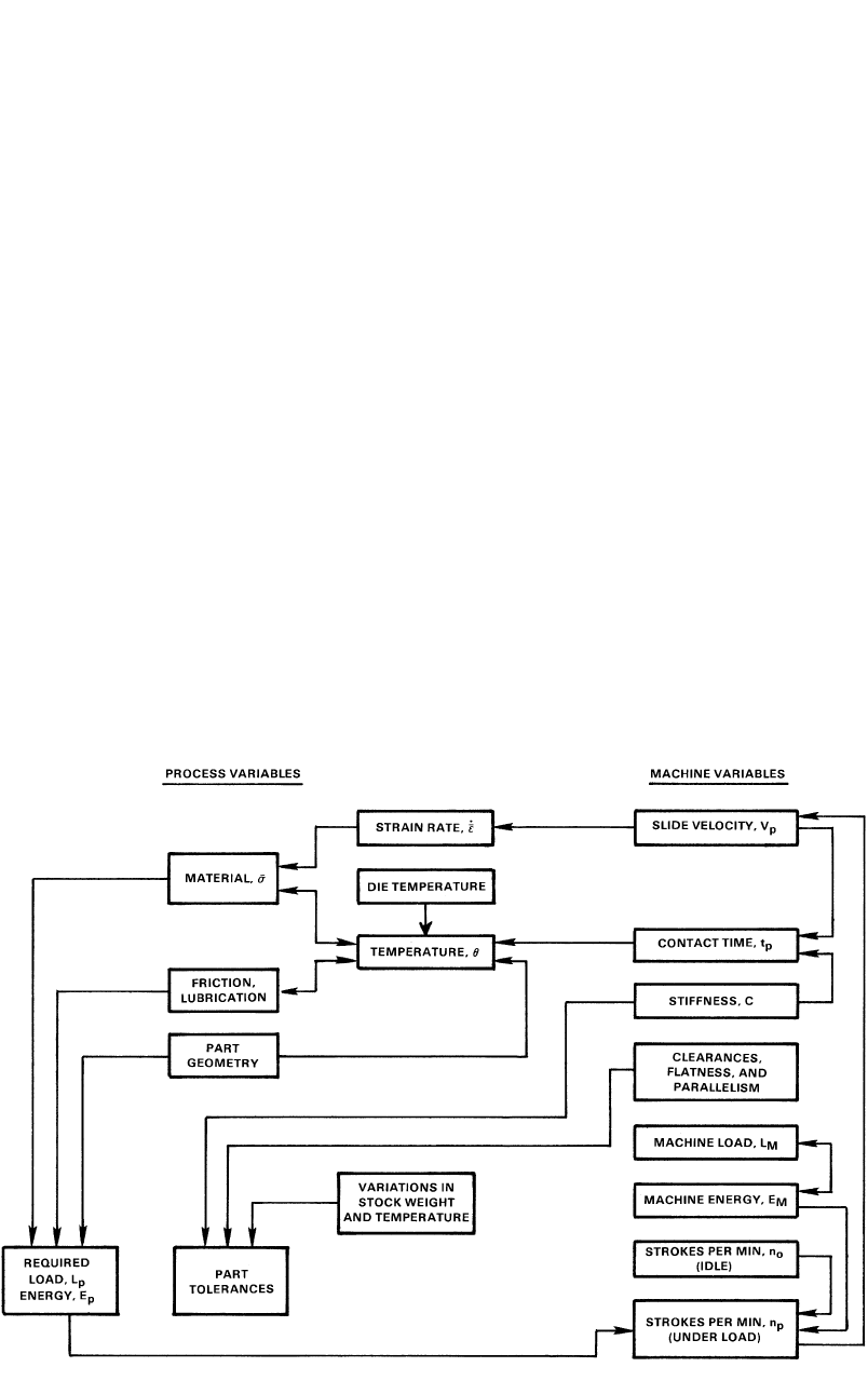
The interaction between the principal ma-

chine and process variables is illustrated in Fig.

10.1 for hot forming processes conducted in

presses. As can be seen in Fig. 10.1, the ﬂow

stress, the interface friction conditions, and¯r,

the forging geometry (dimensions, shape) deter-

mine (a) the load, L

, at each position of the

stroke and (b) the energy, E

, required by the

forming process.

The ﬂow stress, increases with increasing¯r,

deformation rate, and with decreasing tem-

¯e,

perature, h. The magnitudes of these variations

depend on the speciﬁc forming material. The

frictional conditions deteriorate with increasing

die chilling.

As indicated by lines connected to the tem-

perature block, for a given initial stock tempera-

ture, the temperature variations in the part are

largely inﬂuenced by (a) the surface area of con-

tact between the dies and the part, (b) the part

thickness or volume, (c) the die temperature, (d)

the amount of heat generated by deformation

and friction, and (e) the contact time under pres-

sure.

The velocity of the slide under pressure, V

determines mainly the contact time under pres-

sure, t

, and the deformation rate, The number

¯e.

of strokes per minute under no-load conditions,

, the machine energy, E

, and the deformation

energy, E

, required by the process inﬂuence the

slide velocity under load, V

, and the number of

Cold and Hot Forging Fundamentals and Applications

Taylan Altan, Gracious Ngaile, Gangshu Shen, editors, p107-113

DOI:10.1361/chff2005p107

www.asminternational.org

108 / Cold and Hot Forging: Fundamentals and Applications

Fig. 10.1 Relationships between process and machine variables in hot forming process conducted in presses. [Altan et al., 1973]

strokes under load, n

determines the maxi-

mum number of parts formed per minute (i.e.,

the production rate) provided that feeding and

unloading of the machine can be carried out at

that speed.

The relationships illustrated in Fig. 10.1 apply

directly to hot forming of discrete parts in hy-

draulic, mechanical, and screw presses, which

are discussed later. However, in principle, most

of the same relationships apply also in other hot

forming processes such as hot extrusion and hot

rolling.

10.3 Load and Energy

Requirements in Forming

It is useful to consider forming load and en-

ergy as related to forming equipment. For a

given material, a speciﬁc forming operation

(such as closed-die forging with ﬂash, forward,

or backward extrusion, upset forging, bending,

etc.) requires a certain variation of the forming

load over the slide displacement (or stroke). This

fact is illustrated qualitatively in Fig. 10.2,

which shows load versus displacement curves

characteristic of various forming operations.

For a given part geometry, the absolute load

values will vary with the ﬂow stress of the given

material as well as with frictional conditions. In

the forming operation, the equipment must sup-

ply the maximum load as well as the energy re-

quired by the process.

The load-displacement curves, in hot forging

a steel part under different types of forging

equipment, are shown in Fig. 10.3. These curves

illustrate that, due to strain rate and temperature

effects, for the same forging process, different

forging loads and energies are required by dif-

ferent machines. For the hammer, the forging

load is initially higher, due to strain-rate effects,

but the maximum load is lower than for either

hydraulic or screw presses. The reason is that

the extruded ﬂash cools rapidly in the presses,

while in the hammer, the ﬂash temperature re-

mains nearly the same as the initial stock tem-

perature.

Thus, in hot forging, not only the material and

the forged shape, but also the rate of deformation