CIMA - C3 Fundamentals Of Business Mathematics

Подождите немного. Документ загружается.

40 1a: Basic mathematical techniques ⏐ Part A Basic mathematics

Chapter Roundup

• An integer is a whole number and can be either positive or negative.

• Fractions and decimals are ways of showing parts of a whole.

• The negative number rules are as follows.

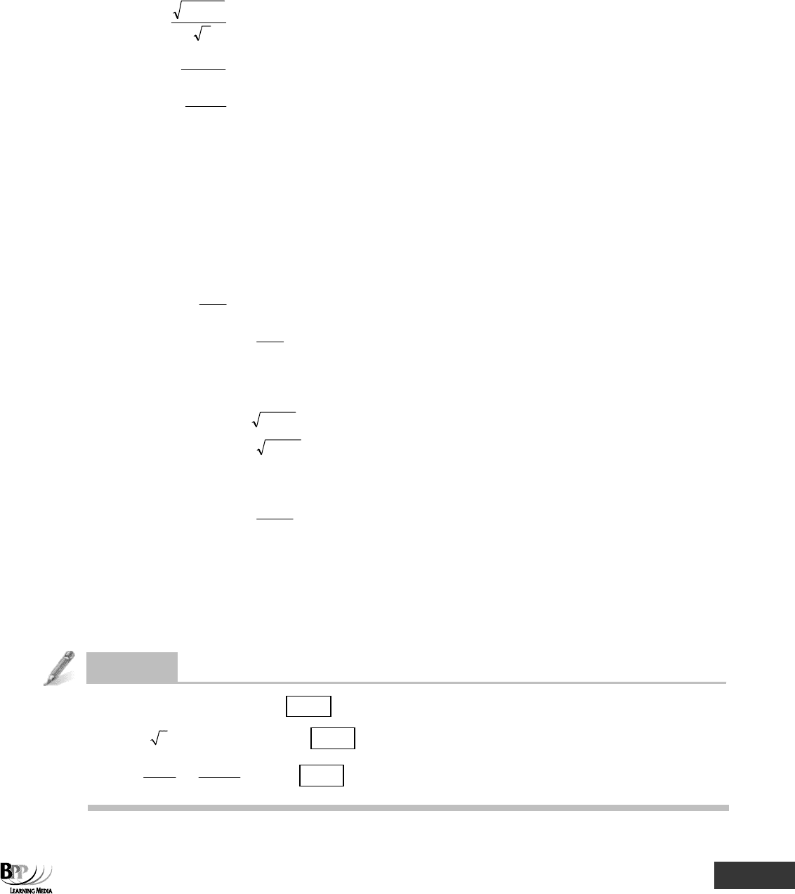
– p + q = q – p

q – (–p) = q + p

– p × –q = pq and

−

–p × q = –pq and

−

=−

• Scientific calculators can make calculations quicker and easier.

• Brackets indicate a priority or an order in which calculations should be made.

• The reciprocal of a number is 1 divided by that number.

• Percentages are used to indicate the relative size or proportion of items, rather than their absolute size. To turn a

percentage into a fraction or decimal you divide by 100%.

• To turn a fraction or decimal back into a percentage you multiply by 100%.

• A percentage increase or reduction is calculated as (change ÷ original value) × 100%.

• A proportion means writing a percentage as a proportion of 1 (that is, as a decimal). 100% can be thought of as

the whole, or 1. 50% is half of that, or 0.5.

• Ratios show relative shares of a whole.

• The n

root of a number is a value which, when multiplied by itself (n–1) times, equals the original number.

Powers work the other way round.

• The main rules to apply when dealing with powers and roots are as follows.

– 2

× 2

= 2

x + y

– 2

÷ 2

= 2

x – y

– (2

)

= 2

– x

= 1

– x

= x

– 1

= 1

– 2

–x

–

133

⎛⎞ ⎛⎞

⎜⎟ ⎜⎟

⎝⎠ ⎝⎠

• If calculations are made using values that have been rounded, then the results of such calculations will be

approximate. The maximum possible error can be calculated.

• A spreadsheet is an electronic piece of paper divided into rows and columns. It is used for calculating, analysing

and manipulating data.

Part A Basic mathematics ⏐ 1a: Basic mathematical techniques 41

Quick Quiz

1 3

is an integer/fraction/decimal

2 1004.002955 to nine significant figures is

3 The product of a negative number and a negative number is

Positive

Negative

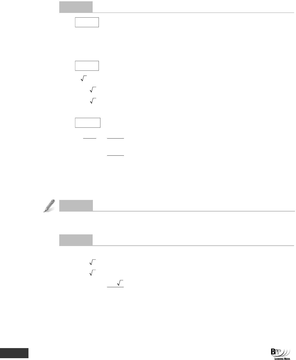
4 What is the value of

2.06 13.051

26.4) ( x 22.034

−−

−

⎟

⎠

⎞

⎜

⎝

⎛

−

2) ( x 33.5

To 2 decimal places?

5 Sales for a business two years ago were $30 million. Last year sales were 8% higher than the year before and this

year, sales were 6% higher than last year. What are this year's sales? (correct to 3 significant figures)

6 3

–1

can also be written as

A 3

–1

B 3

D –1

7 The cost of materials for a component is $20.00 to the nearest $1. What is the maximum absolute error in the

cost?

8 The expression

(X )

equals.

A X

B I

C O

D X

9 An employee does not pay tax on the first $4,000 of earnings and then 25% tax on the rest of earnings. If he wants

to have $20,000 net of tax earnings, what gross earnings (to the nearest $) does he need? $

10 You are about to key an exam mark into cell B4 of a spreadsheet. Write an IF statement to be placed in cell C4, that

will display PASS in C4 if the student mark is 50 or above and, will display FAIL if the mark is below 50.

42 1a: Basic mathematical techniques ⏐ Part A Basic mathematics

Answers to Quick Quiz

1 Fraction

2 1004.00296

3 Positive

;

4 37.48

5 34.3

Sales 2 years ago = $30m

Sales 1 year ago = $30m + 8%

= $30m × 1.08

= $32.4m

Sales this year = $32.4 + 6%

= $32.4 × 1/06

= 34.344

= 34.3 (3 sf)

6 C =

7 50c

8 A

(X )

= X

9 $

Taxable part of earnings = 20,000 – 4,000

= $16,000

Taxable earnings =

0.25)(1

16,000

−

= $21,333

Gross earnings = $21,333 + $4,000

= $25,333

10 = IF (B4>49,"PASS","FAIL")

Now try the questions below from the Exam Question Bank

Question numbers Page

1–16 325-328

25,333

Topic list Syllabus references

1 Formulae and equations A, (i), (iv), (1)

2 Manipulating inequalities A, (5)

3 Linear equations A, (iv)

4 Linear equations and graphs A, (v)

5 Simultaneous equations A, (iv), (4)

6 Non-linear equations A, (iv), (v), (4)

7 Using spreadsheets to produce graphs G (i) (1)

Formulae and

equations

Introduction

Many formulae and equations appear in financial and business calculations and being able to

deal with them is an essential skill.

Many students get confused when they have to deal with mathematical symbols and letters

but they are simply a shorthand method of expressing words.

Graphs can be used to illustrate equations and this chapter will show you how to draw them

manually and using spreadsheets.

44 1b: Formulae and equations ⏐ Part A Basic mathematics

1 Formulae and equations

1.1 Formulae

So far all our problems have been formulated entirely in terms of specific numbers. However, we also need to be

able to use letters to represent numbers in formulae and equations.

A formula enables us to calculate the value of one variable from the value(s) of one or more other variables.

1.1.1 Use of variables

The use of variables enables us to state general truths about mathematics and you will come across many

formulae in your CIMA studies.

For example:

• x = x

• x

= x × x

• If y = 0.5 × x, then x = 2 × y

These will be true whatever values x and y have. For example, let y = 0.5 × x

• If y = 3, x = 2 × y = 6

• If y = 7, x = 2 × y = 14

• If y = 1, x = 2 × y = 2, and so on for any other choice of a value for y.

We can use variables to build up useful formulae, we can then put in values for the variables, and get out a value

for something we are interested in. It is usual when writing formulae to leave out multiplication signs between

letters. Thus p × u – c can be written as pu – c. We will also write (for example) 2x instead of 2 × x.

1.1.2 Example: Variables

For a business, profit = revenue – costs. Since revenue = selling price × units sold, we can say that:

profit = (selling price × units sold) – costs.

'(Selling price × units sold) – costs' is a formula for profit.

Notice the use of brackets to help with the order of operations.

We can then use single letters to make the formula quicker to write.

Let p = profit

s = selling price

u = units sold

c = cost

Then p = (s × u) – c.

If we are then told that in a particular month, s = $5, u = 30 and c = $118, we can find out the month's profit.

Profit = p = (s × u) – c = ($5 × 30) – $118

= $150 – $118 = $32

T F

RWAR

Part A Basic mathematics ⏐ 1b: Formulae and equations 45

1.1.3 Example: A more complicated formula

In your later CIMA studies, you will come across the learning curve formula, Y = aX

which shows how unit labour

times tend to decrease at a constant rate as production increases.

Y = cumulative average time taken per unit

a = time taken for the first unit

X = total number of units

b = index of learning

What is the average time taken per unit if the time taken for the first unit is 10 minutes, the total number of units is

8 and the index of learning is – 0.32?

Solution

Y = aX

a = 10 minutes

X = 8

b = – 0.32

Y = 10 × 8

– 0.32

= 5.14

On your calculator, press 10 × 8 X (–) 0.32 =

1.2 Equations

In the above example, su – c was a formula for profit. If we write p = su – c, we have written an equation. It says

that one thing (profit, p) is equal to another (su – c).

1.2.1 'Solving the equation'

Sometimes, we are given an equation with numbers filled in for all but one of the variables. The problem is then to

find the number which should be filled in for the last variable. This is called solving the equation.

(a) Returning to p = su – c, we could be told that for a particular month s = $4, u = 60 and c = $208. We

would then have the equation p = ($4 × 60) – $208. We can solve this easily by working out ($4 ×

60) – $208 = $240 – $208 = $32. Thus p = $32.

(b) On the other hand, we might have been told that in a month when profits were $172, 50 units were

sold and the selling price was $7. The thing we have not been told is the month's costs, c. We can

work out c by writing out the equation.

$172 = ($7 × 50) – c

$172 = $350 – c

error, we can get to c = $178.

46 1b: Formulae and equations ⏐ Part A Basic mathematics

1.2.2 The rule for solving equations

The general rule for solving equations is that you must always do the same thing to both sides of the equal sign

so the 'scales' stay balanced.

(a) To solve an equation, we need to get it into the following form.

Unknown variable = something with just numbers in it, which we can work out.

We therefore want to get the unknown variable on one side of the = sign, and everything else on the

other side.

(b) The rule is that you must always do the same thing to both sides of the equal sign so the 'scales'

stay balanced. The two sides are equal, and they will stay equal so long as you treat them in the

same way.

$172 + c = $350

Take $172 from both sides: $172 + c –$172 = $350 – $172

c = $350–$172

c = $178

1.2.3 Example: Solving the equation

For example, you can do any of the following: add 37 to both sides; subtract 3x from both sides; multiply both

sides by –4.329; divide both sides by (x + 2); take the reciprocal of both sides; square both sides; take the cube

root of both sides.

We can do any of these things to an equation either before or after filling in numbers for the variables for which we

have values.

(a) If $172 = $350 – c (as in Paragraph 1.2.1) we can then get

$172 + c = $350 (add c to each side)

c = $350 – $172 (subtract $172 from each side)

c = $178 (work out the right hand side)

(b) 450 = 3x + 72 (initial equation: x unknown)

450 – 72 = 3x (subtract 72 from each side)

72450 −

= x (divide each side by 3)

126 = x (work out the left hand side)

– $172

–

$172

T F

RWAR

Part A Basic mathematics ⏐ 1b: Formulae and equations 47

3y + 9 = 5y (add 7 to each side)

9 = 2y (subtract 3y from each side)

4.5 = y (divide each side by 2)

(d)

xx3

= 7 (initial equation: x unknown)

xx3

= 49 (square each side)

()

1x3 +

= 49 (cancel x in the numerator and the denominator of the left hand

side: this does not affect the value of the left hand side, so we do

not need to change the right hand side)

3x + 1 = 196 (multiply each side by 4)

3x = 195 (subtract 1 from each side)

x = 65 (divide each side by 3)

(e) Our example in Paragraph 1.2 was p = su – c. We could change this, so as to give a formula for s.

s = su – c

p + c = su (add c to each side)

cp +

= s (divide each side by u)

s =

cp +

(swap the sides for ease of reading)

Given values for p, c and u we can now find s. We have rearranged the equation to give s in terms of

p, c and u.

(f) Given that y =

7x3 + , we can get an equation giving x in terms of y.

y =

7x3 +

= 3x + 7 (square each side)

– 7 = 3x (subtract 7 from each side)

x =

−

(divide each side by 3, and swap the sides for ease of reading)

1.2.4 Solving the equation and brackets

In equations, you may come across expressions like 3(x + 4y – 2) (that is, 3 × (x + 4y – 2)). These can be re-

written in separate bits without the brackets, simply by multiplying the number outside the brackets by each item

inside them. Thus 3(x + 4y – 2) = 3x + 12y – 6.

Question

Solving the equation (1)

(a) If 47x + 256 = 52x, then x =

(b) If 4 x + 32 = 40.6718, then x =

3x 4 2.7x 2

+−

, then x =

48 1b: Formulae and equations ⏐ Part A Basic mathematics

Answe

(a)

x = 51.2

47x + 256 = 52x

256 = 5x (subtract 47x from each side)

51.2 = x (divide each side by 5)

(b)

x = 4.7

x4 + 32 = 40.6718

= 8.6718 (subtract 32 from each side)

x = 2.16795 (divide each side by 4)

x = 4.7 (square each side).

(c)

x = –1.789

4x3

2x7.2

−

3x + 4 =

2x7.2 −

(take the reciprocal of each side)

15x + 20 = 2.7x – 2 (multiply each side by 5)

12.3x = – 22 (subtract 20 and subtract 2.7x from each side)

x = – 1.789 (divide each side by 12.3).

Question

Solving the equation (2)

(a) Rearrange x = (3y – 20)

to get an expression for y in terms of x.

(b) Rearrange 2(y – 4) – 4(x

+ 3) = 0 to get an expression for x in terms of y.

Answe

(a) x = (3y – 20)

x = 3y – 20 (take the square root of each side)

20 + x = 3y (add 20 to each side)

y =

x20 +

(divide each side by 3, and swap the sides for ease of reading)

(b) 2(y – 4) – 4(x

+ 3) = 0

2(y – 4) = 4 (x

+ 3) (add 4(x

+ 3) to each side)

0.5(y – 4) = x

+ 3 (divide each side by 4)

0.5(y – 4) – 3 = x

(subtract 3 from each side)

Part A Basic mathematics ⏐ 1b: Formulae and equations 49

x = 3)4(y5.0 −− (take the square root of each side, and swap the sides for ease

of reading)

x =

5y5.0 −

2 Manipulating inequalities

An inequality is a statement that shows the relationship between two (or more) expressions with one of the

following signs: >, .,<, -. We can solve inequalities in the same way that we can solve equations.

2.1 Inequality symbols

Equations are called inequalities when the '=' sign is replaced by one of the following.

(a) > means 'greater than'

(b) . means 'is greater than or equal to'

(d) - means 'is less than or equal to'+

2.2 Using inequalities

Inequalities are used in a short-term decision making technique called linear programming which you will come

across in your managerial studies. It involves using inequalities to represent situations where resources are

limited.

2.2.1 Example: Using inequalities 1

If a product needs 3kg of material and 700 kg is available, express this as an inequality

Solution

If the number of units of the product = X

3X - 700

2.2.2 Example: Using inequalities 2

Product Z needs 3 minutes of machining time and product Y needs 2 minutes of machining time. There are 10

hours of machining time available. Express this as an inequality.

Solution

10 hours of machining time = 600 minutes

The total machining time must be less than or equal to 600 minutes.

3Z + 2Y- 600

where Z = no of units of product Z

Y = no of units of product Y

T F

RWAR