Chung Y.-W. Practical guide to surface science and spectroscopy
Подождите немного. Документ загружается.


47
3.2 PHOTON SOURCES
3.2 PHOTON SOURCES
A list of commonly available laboratory light sources is shown as
follows:
Photon source Energy (eV) Natural width (eV)
Ti K␣
1
4511 1.4
Al K␣
1,2
1486.6 0.9
Mg K␣
1,2
1253.6 0.8
Na K␣
1,2
1041 0.7
Zr M 151.4 0.8
YM 132.3 0.5
HeII 40.8 ⬍ 0.01
NeII 26.9 ⬍ 0.01
HeI 21.22 ⬍ 0.01
NeI 16.85, 16.67 ⬍ 0.01
Ar 11.83, 11.62 ⬍ 0.01
H 10.2 ⬍ 0.01
Except for the Zr and Y sources, there is a wide gap between 40 eV
and 1000 eV. Therefore, photoelectron spectroscopy is conventionally
divided into two regimes: X-ray photoelectron spectroscopy (XPS) or
ESCA (electron spectroscopy for chemical analysis), and ultraviolet
photoelectron spectroscopy (UPS). In XPS, the most commonly used
photon sources are the Al and Mg K␣ lines. The most commonly used
sources in UPS are the HeI and HeII lines.
X-ray yield using an Al or Mg anode is low because of their low
atomic number, typically 10
-3
photon per electron per steradian at 10
keV. To maximize the photoelectron signal, the X-ray source is brought
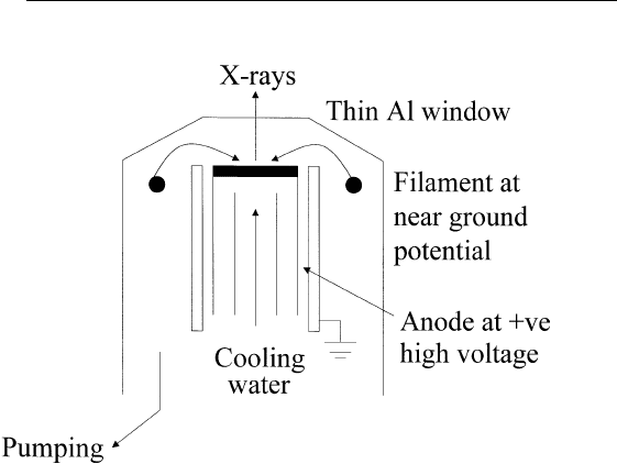
close to the sample surface. A typical construction is shown in Fig.
3.2. In this design, a thoriated tungsten filament is biased at near ground
potential and heated to emit electrons. The anode is biased at positive
high voltage. The two grounding shields serve to focus the electrons
to the anode. There is no direct line of sight from filament to anode
to prevent anode contamination. The anode must be electrically isolated
and water-cooled. A thin window (typically an Al window with thick-
ness on the order of a few micrometers) is incorporated to cut off stray
electrons and minimize bremsstrahlung. Additional pumping may be
needed to minimize pressure rise in the X-ray source due to outgassing
(which can result in arcing and destruction of the thin window).
48
CHAPTER 3 / PHOTOELECTRON SPECTROSCOPY
FIGURE 3.2 Typical construction of an X-ray source for XPS studies.
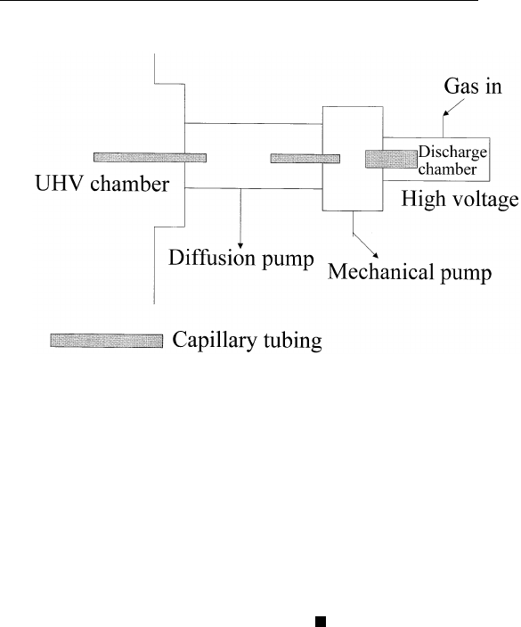
Intense UV lines are generated by gas discharge at pressures be-
tween 0.1 and 1 torr. For UPS work at photon energies less than 11.6
eV, a LiF window can be used to transmit the light from the source to
the sample inside the UHV chamber. No window material is available
to transmit photons with energies above 11.6 eV. To maintain the gas
discharge in the light source (0.1–1 torr) and the vacuum integrity of
the UHV chamber (10
⫺9
torr or better), one has to use a differential
pumping technique. Here, the pressure at the UV source is reduced
sequentially through two or three stages to 10
⫺9
torr or below in the
UHV chamber. This is shown schematically in Fig. 3.3.
E
XAMPLE.
This is an illustration of the principle of differential
pumping. Consider a capillary tubing of length L and inner diameter
D. When a pressure difference dP is established across the length of
this tube, the gas flow rate S (in liter-torr/s) is given by dP (torr) ⫻
C (liters/s), where C is known as the conductance. Note the analogy
of this formula to Ohm’s Law. C is given by 12.0 (D
3
/L) liters/sec, D
and L in centimeters. For a tubing of length 10 cm and inner diameter
0.1 cm, what is the maximum gas flow rate at a pressure differential
of 100 Torr across this tubing? If the low-pressure end of the tubing
is evacuated by a pump of speed 10 liters/s at a pressure of 10
⫺9
torr,
what is the pressure at the other end of the tubing?
49
3.2 PHOTON SOURCES
FIGURE 3.3 Typical construction of a windowless UV source for UPS studies.
S
OLUTION.
The conductance of the given tubing is equal to 12.0
⫻ (0.001/10) ⫽ 1.2 ⫻ 10
⫺3
liter/s. For dP ⫽ 100 torr, the gas flow
rate S ⫽ (100) ⫻ (1.2 ⫻ 10
⫺3
) ⫽ 0.12 liter-Torr/sec.
If the low-pressure end of the tubing is at 10
⫺9
Torr with a pump
of speed 10 liters/s, the gas removal rate ⫽ (10
⫺9
) ⫻ (10) ⫽ 10
⫺8
liter-torr/s. From the known conductance of the tubing, we can calculate
the pressure differential as (10
⫺8
)/(1.2 ⫻ 10
⫺3
) ⫽ 0.83 ⫻ 10
⫺5
torr.
Therefore, the pressure at the other end of the tubing ⫽ (0.83 ⫻ 10
⫺5
⫹ 10
⫺9
) torr ⫽ 0.83 ⫻ 10
⫺5
torr.
In order to have the maximum flexibility in a given experiment,
the photon source should ideally be monochromatic and polarized, have
variable energy, and be of sufficient intensity. Sources listed earlier
fulfill some but not all of these qualifications, especially tunability. The
only photon source satisfying all these requirements is the synchrotron
radiation source.
When electrons (or any charged particles) travel at constant speed
in a circle, they are subjected to centripetal acceleration. As a result
of this acceleration, electromagnetic radiation is emitted. When elec-
trons are moving in a circle at speeds v close to the speed of light c,
electromagnetic radiation is emitted as a narrow beam along the tangent
of the circle and is almost completely polarized in the plane of motion.
This is known as synchrotron radiation. When v ⬇ c, the emitted
radiation covers an energy range given approximately by ␥
3
ប
o
where

50
CHAPTER 3 / PHOTOELECTRON SPECTROSCOPY
␥ ⫽ (1 ⫺ v
2
/c
2
)
⫺1/2
⫽ ratio of electron mass to its rest mass (m/m
o
),
and
o
the orbital angular frequency.
E
XAMPLE.
Consider the 7-GeV Advanced Photon Source at Ar-
gonne National Laboratory. In a curved section of this synchrotron
with local radius equal to 30 m, calculate the energy range of the
synchrotron radiation.
S
OLUTION.
The 7-GeV designation means that the electron energy
is equal to 7 GeV. Therefore,
␥
is equal to 7000/0.5 ⫽ 14,000, since
the electron rest mass is equal to 0.5 MeV. At these energies, the speed
of electrons is effectively the speed of light (⫽ 3 ⫻ 10
8
m/s). For a
local radius of 30 m, the angular frequency
o
⫽ 3 ⫻ 10
8
/30⫽ 10
7
/
sec. The energy range of synchrotron radiation is then equal to
␥
3
ប
o
⫽ (14000)
3.
(1.05 ⫻ 10
⫺34
) (10
7
) / 1.6 ⫻ 10
⫺19
eV ⫽ 18 keV.
Q
UESTION FOR
D
ISCUSSION.
What are the major advantages and
disadvantages of using synchrotron radiation?
3.3 DETECTORS
Most photoelectron spectrometers are of the band-pass type. With labo-
ratory photon sources, typical photoelectron signals are on the order
of a few hundred to a few hundred thousand electrons per second
(10
⫺17
to 10
⫺14
A). Such small signals are normally detected by electron
counting: The photoelectrons impinge on an electron multiplier that is
set to give a gain on the order of 10
5
, that is, for each electron entering
the multiplier, a charge pulse containing 10
5
electrons will emerge at
the output end of the multiplier. The electron pulse is amplified further
and counted by standard counting electronics
1
. In some cases, parallel
detection using an electron multiplier array is used to increase the
effective data rate. Also, electron optics are sometimes used to collect
photoelectron signals from areas as small as 1–10 microns.
1
At a multiplier gain of 10
5
, the total charge is 1.6 ⫻ 10
⫺14
C. When this charge
falls on a capacitor (as in the case of a field effect transistor), one obtains a stepwise
increase in voltage dV. For capacitance ⫽ 1pF,dV ⫽ 0.016 V. This voltage signal
can be readily conditioned and amplified for further processing. Counting electronics
can be set to discriminate against signals that are too low (background noise) or too
high (occasional glitches). Most counting electronics can handle signals up to ⬃1 ⫻
10
6
per second.

51
3.5 CHEMICAL SHIFT
3.4 ELEMENT IDENTIFICATION
Typically, the Mg or Al K␣ source is used for XPS studies in the
laboratory. This X-ray photon energy is sufficient to excite electrons
from most core levels of interest. Subsequent relaxation within the
excited ion can result in the emission of Auger electrons. Therefore, an
X-ray photoelectron spectrum contains Auger information for element
identification purposes. In addition, core levels of atoms have well-
defined binding energies. Therefore, element identification can also be
accomplished by locating these core levels. Because of the ability of
X-ray photoelectron spectroscopy to identify elements, this technique
is also known as ESCA (electron spectroscopy for chemical analysis).
The typical number sensitivity of ESCA is about the same order
of electron-excited Auger electron spectroscopy, ⬃ 0.1–1% of a mono-
layer. The advantage of XPS is twofold: (i) X-ray photons appear to
be less damaging to surfaces than electrons; (ii) the X-ray photoelectron
spectrum contains chemical state information that is sometimes more
easily interpreted than the corresponding Auger electron spectrum.
Q
UESTION FOR
D
ISCUSSION.
In a typical XPS spectrum, peaks due
to Auger electrons and photoelectron emission from core levels are
observed. How does one distinguish between them?
3.5 CHEMICAL SHIFT
Consider a free atom of sodium whose electronic configuration is
ls
2
2s
2
2p
6
3s
1
. Let us assume that sodium participates in a certain chemi-
cal reaction in which the outermost valence electron is removed, such
as Na reacting with Cl to give Na
⫹
Cl
⫺
. All remaining electrons in the
sodium ion will be moving in a more positive potential. As a result,
core-level binding energies will increase. This is known as chemical
shift. For transition metals that exhibit multiple oxidation states, one
can correlate the binding energy shift and the oxidation state. For
example, the Cu 2p
3/2
core level binding energies are 932.8, 934.7,
and 936.2 eV in pure Cu, Cu
2
O and CuO respectively. Chemical shifts
are typically on the order of electron volts.
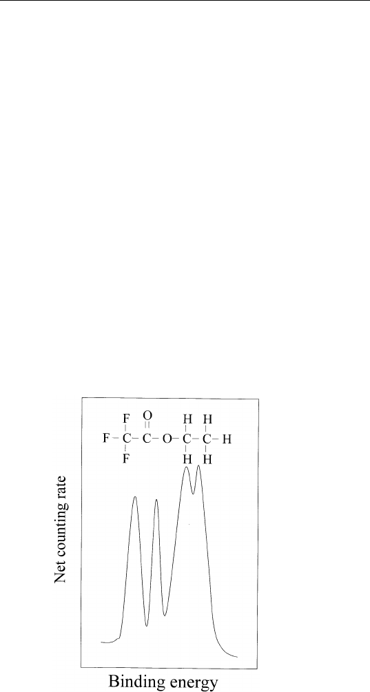
Chemical shift analysis can be used to study nearest neighbor
environments in molecules or solids. An excellent example is illustrated
for the molecule CF
3
COOC
2
H
5
(ethyl fluoroacetate). The four carbon
52
CHAPTER 3 / PHOTOELECTRON SPECTROSCOPY
atoms are located in environments different from one another (see Fig.
3.4). The first carbon atom from the left is surrounded by three fluorine
atoms. Fluorine is the most electronegative element and tends to draw
electrons from the carbon atom, making the latter slightly positively
charged. Oxygen is also very electronegative and the attached carbon
atom is charged positively, but not as much as the first one. The third
carbon atom is bonded to two hydrogen atoms and another oxygen.
But carbon is slightly more electronegative than hydrogen. This results
in an almost neutral carbon atom. The fourth carbon atom is subjected
to the influence of three hydrogen atoms and is expected to be slightly
negatively charged. It has the smallest ls binding energy among the
four carbon atoms as shown in Fig. 3.4.
Chemical shift is also seen in AES. For an Auger WXY transition,
the energy of the Auger electron is E
W
⫺ E
X
⫺ E
Y
(not including the
work function term). Any change in the Auger electron energy is due
to the net effect of chemical shifts of the three levels W, X, and Z,
which are not necessarily identical. This makes interpretation more
difficult.
FIGURE 3.4 Carbon 1s spectrum for ethyl fluoroacetate. The four different chemi-
cal states of carbon atoms are clearly identified.

53
3.6 RELAXATION SHIFT AND MULTIPLET SPLITTING
3.6 RELAXATION SHIFT AND MULTIPLET SPLITTING
A phenomenon called relaxation complicates the simple chemical shift
analysis. For example, when an inert gas atom is implanted into different
metals such as gold, silver, and copper, the measured binding energy
of a given core level of the inert gas atom depends on the surrounding
medium. Since chemical bonding is not expected, the observed binding
energy shift has to be interpreted differently. In the photoionization
process, the outgoing photoelectron and the electron vacancy or hole
left behind have an attractive interaction. Electrons in the surrounding
medium relax toward this hole, thus partially screening such attractive
interaction. This relaxation results in a higher measured kinetic energy
of the photoelectron (or smaller apparent binding energy) than when
relaxation is absent. Since relaxation depends on the surrounding me-
dium, the measured binding energy also depends on the medium. Such
an apparent shift in the absence of chemical bonding is known as
relaxation shift.
The necessity of considering relaxation shift is due to the many-
electron nature of the photoelectron emission process. When an electron
is photoemitted from an N-electron system (an atom or a solid), the
resulting (N⫺1) electrons move in a different potential and adjust
themselves to a lower total energy (i.e., the electron orbitals are not
frozen). This adjustment is the relaxation shift.
Another effect of the many-electron nature of photoemission is
multiplet splitting. Consider the example of photoemission from the
1s orbital of a lithium atom, which has an electronic configuration of
ls
2
2s
1
. After photoemission of the 1s electron, we have an Li
⫹
ion,
as follows:
Li ⫹ h
→ Li
⫹
⫹ e. (3.2)
By energy conservation, the kinetic energy of the photoelectron E
kin
is given by
E
kin
⫽ h
⫹ E(Li) ⫺ E(Li
⫹
). (3.3)
There are two possible electronic configurations for Li
⫹
(1s
1
2s
1
). The
two electrons can have parallel (triplet state) or antiparallel (singlet
state) spins. Therefore, one can observe two photoelectron peaks due
to photoemission from the 1s level of lithium.
54
CHAPTER 3 / PHOTOELECTRON SPECTROSCOPY
3.7 CHEMICAL BONDING ON SURFACES
Many surface chemical reactions such as those in oxidation and catalysis
do not occur as one-step processes. They may go through a number
of steps with the formation of intermediate compounds or complexes
before the final products are released. In many cases, photoelectron
spectroscopy provides direct information on the chemical state of the
surface in the course of the reaction; in some cases, even the orientation
of molecules adsorbed on surfaces can be deduced. Let us look at three
examples:
E
XAMPLE
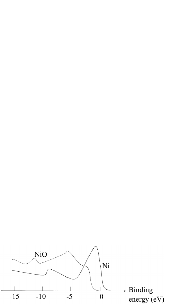
1. Oxidation of Nickel. Nickel is a metal and therefore
has a nonzero density of states at the Fermi level (Fig. 3.5). When it
is oxidized, electrons are transferred from the metal to the oxygen 2p
level, located at 6–8 eV below the Fermi level. The photoelectron
spectrum shows that this surface oxide is a nonmetal because there is
no density of electrons at the Fermi level. The O(2p) orbital is clearly
visible.
E
XAMPLE
2. Dehydrogenation of Ethylene (C
2
H
4
) to Acetylene
(C
2
H
2
). When acetylene (C
2
H
2
) is adsorbed onto a clean nickel at 100
K, it gives rise to additional photoelectron emission on top of the
emission from nickel. This extra emission due to acetylene can be
observed more clearly by taking the difference between the spectrum
from the surface with acetylene and without. The resulting difference
spectrum N(E) is shown in Fig. 3.6a and is similar to that obtained
from gas phase acetylene, except for a slight shift of the
-orbital
toward larger binding energy. This shows that acetylene stays intact
when adsorbed onto nickel at 100 K. The same is also true when
FIGURE 3.5 UPS spectrum of clean Ni and NiO surfaces.
55
3.7 CHEMICAL BONDING ON SURFACES
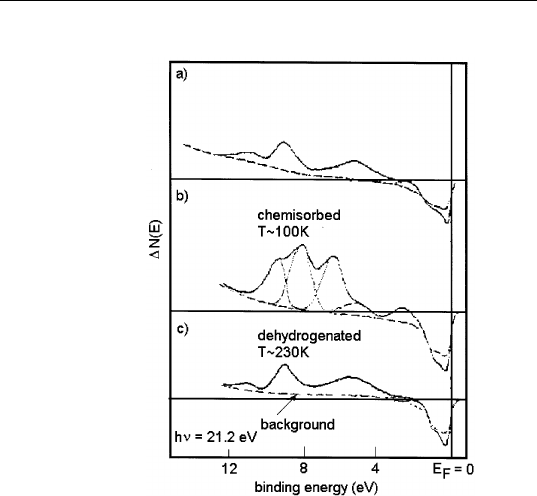
FIGURE 3.6 UPS difference spectrum for Ni after (a) 1.2 L exposure to acetylene
at 100 K, (b) 1.2 L exposure to ethylene at 100 K, and (c) after surface warmed to
230 K. (Adapted from J. E. Demuth and D. E. Eastman, Phys. Rev. Lett. 32, 1123
(1974).)
ethylene is adsorbed onto clean nickel at 100 K (Fig. 3.6b). However,
when the latter surface is warmed up to 230 K or higher, the difference
spectrum changes to that shown in Fig. 3.6c and is identical to that
of acetylene adsorbed on Ni at 100 K. This indicates that ethylene
dehydrogenates to acetylene at 230 K.
E
XAMPLE
3. Orientation of CO on Ni(100). Example 2 is the most
typical way in which photoelectron spectroscopy is being used in surface
chemical studies. This is essentially a fingerprinting technique. One
simply compares the photoelectron difference spectrum obtained with
that of a gas-phase molecule. In some cases, photoelectron spectroscopy
goes beyond this fingerprinting application and is used to identify the
possible orientation of molecules on metal surfaces. The basic idea is
that the various molecular orbitals of a given molecule are highly
directional and have different symmetries. One would thus expect that
the probability of ejecting an electron by a photon is a function of
direction.
56
CHAPTER 3 / PHOTOELECTRON SPECTROSCOPY
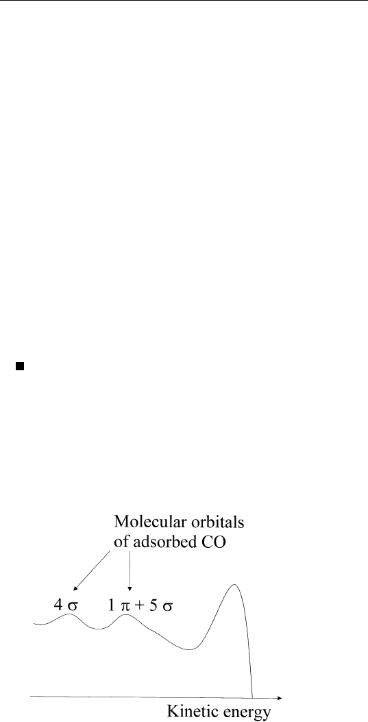
When CO is adsorbed onto Ni(100), it gives rise to two extra
emissions at about 9 and 11 eV below the Fermi level due to the 1
⫹ 5
and 4
molecular orbitals of CO, respectively (Fig. 3.7). At
h
⬃ 35 eV, these two peaks attain maximum intensity (known as
‘‘resonance’’). It is shown theoretically that this resonance is due to
emission into a final state with
symmetry (i.e., cylindrical symmetry
about the C–O axis). The theory also predicts that a
-initial state can
only emit to this final state with the electric field vector A (of the incident
electromagnetic radiation) component parallel to the molecular axis.
A
-level, on the other hand, can only emit to this final state with an
A-vector component perpendicular to the molecular axis. Therefore,
when one performs photoemission with a photon energy ⬃ 35 eV, the
angular distribution of the levels due to A
//
(i.e., the component of the
electric field vector parallel to the C–O molecular axis) should be
strongly peaked along the C–O axis. This is shown in Fig. 3.8 for the
4 orbital of CO as a function of angle from the surface normal. As
can be seen, the CO axis is perpendicular to the surface to within 5
o
.
Please refer to Chemical Physics Letters 47, 127 (1977) for further
details.
3.8 BAND STRUCTURE STUDIES
The simplest physical model to describe the photoemission process
from solids is the three-step model: (1) excitation of electrons from
FIGURE 3.7 UPS spectrum of CO on Ni(100).