Chow T.L. Mathematical Methods for Physicists: A Concise Introduction
Подождите немного. Документ загружается.

Solution: Here f xx
2
ÿ 2. Take x
1
1and 0:001, then Eq. (13.13) gives
x
2
1:499750125;
x
3
1:416680519;
x
4
1:414216580;
x
5
1:414213563;
x
6
1:414113562
x
7
1:414113562
)
x
6
x
7
:
Numerical integration
Very often de®nite integrations cannot be done in closed form. When this happens
we need some simple and useful techniques for approximating de®nite integrals.
In this section we discuss three such simple and useful methods .
The rectangular rule
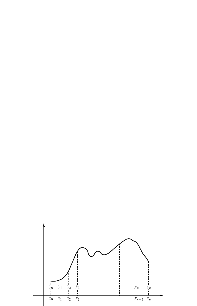
The reader is familiar with the interpretation of the de®nite integral
R
b
a
f xdx as
the area under the curve y f x between the limits x a and x b:
Z
b
a
f xdx
X
n
i1
f
i
x
i
ÿ x
iÿ1
;
where x
iÿ1
i
x
i
; a x
0
< x
1
< x
2
< < x
n
b: We can obtain a good
approximation to this de®nite integral by simply evaluating such an area under
the curve y f x. We can divide the interval a x b into n subintervals of
length h b ÿ a=n, and in each subinterval, the function f
i
is replaced by a
466
NUMERICAL METHODS
Figure 13.5.
straight line connecting the values at each head or end of the subinterval (or at the
center point of the interval), as shown in Fig. 13.5. If we choose the head,
i
x
iÿ1
, then we have
Z
b
a
f xdx hy
0
y
1
y
nÿ1
; 13:14
where y
0
f x
0
; y
1
f x
1
; ...; y
nÿ1
f x
nÿ1
. This method is called the rec-
tangular rule.
It will be shown later that the error decreases as n
2
. Thus, as n increases, the
error decreases rapidly.
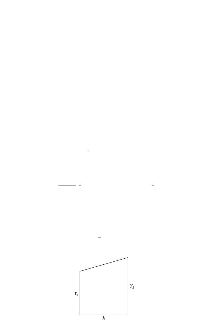
The trapezoidal rule
The trapezoidal rule evaluates the small area of a subinterval slightly diÿerently.
The area of a trapezoid as shown in Fig. 13.6 is given by
1
2
hY
1
Y
2
:
Thus, applied to Fig. 13.5, we have the approximation
Z
b
a
f xdx
b ÿ a
n
1
2
y
0
y
1
y
2
y
nÿ1
1
2
y
n
: 13:15
What are the upper and lower limits on the error of this method? Let us ®rst
calculate the error for a single subinterval of length h b ÿ a=n. Writing
x
i
h z and "
i
z for the error, we have
Z
z
x
i
f xdx
h
2
y
i
y
z
"
i
z;
467
NUMERICAL INTEGRATION
Figure 13.6.
where y
i
f x
i
; yz f z.Or
"
i
z
Z
z
x
i
f xdx ÿ
h
2
f x
i
ÿf z
Z
z
x
i
f xdx ÿ
z ÿ x
i
2
f x
i
ÿf z:
Diÿerentiating with respect to z:
"
0
i
zf zÿf x
i
f z=2 ÿz ÿ x
i
f
0
z=2:
Diÿerentiating once again,
"
00
i
zÿz ÿ x
i
f
00
z=2:
If m
i
and M
i
are, respectively, the minimum and the maximum values of f
00
z in
the subinterval [x
i
; z], we can write
z ÿ x
i
2
m
i
ÿ"
00
i
z
z ÿ x
i
2
M
i
:
Anti-diÿerentiation gives
z ÿ x
i
2
4
m
i
ÿ"
0
i
z
z ÿ x
i
2
4
M
i
Anti-diÿerentiation once more gives
z ÿ x
i
3
12
m
i
ÿ"
i
z
z ÿ x
i
3
12
M
i
:
or, since z ÿ x
i
h,
h
3
12
m
i
ÿ"
i
h
3
12
M
i
:
If m and M are, respectively, the minimum and the maximum of f
00
z in the
interval [a; b] then
h
3
12
m ÿ"
i
h
3
12
M for all i:
Adding the errors for all subintervals, we obtain
h
3
12
nm ÿ"
h
3
12
nM
or, since h b ÿ a=n;
b ÿ a
3
12n
2
m ÿ"
b ÿ a
3
12n
2
M: 13:16
468
NUMERICAL METHODS
Thus, the error decreases rapidly as n increases, at least for twice-diÿerentiable
functions.
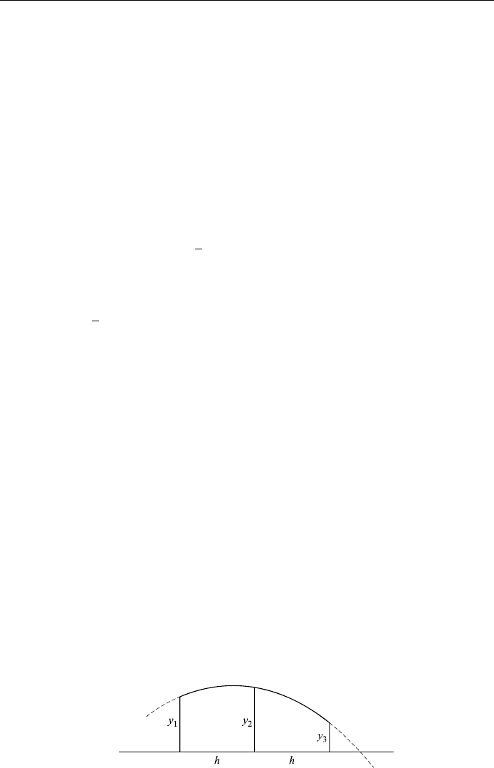
Simpson's rule
Simpson's rule provides a more accurate and useful formula for approximating a
de®nite integral. The interval a x b is subdivided into an even number of
subintervals. A parabola is ®tted to points a, a h, a 2h; another to a 2h,
a 3h, a 4h; and so on. The area under a parabola, as shown in Fig. 13.7, is
(Problem 13.8)
h
3
y
1
4y
2
y
3
:
Thus, applied to Fig. 13.5, we have the approximation
Z
b
a
f xdx
h
3
y
0
4y
1
2y
2
4y
3
2y
4
2y
nÿ2
4y
nÿ1
y
n
; 13:17
with n even and h b ÿ a=n.
The analysis of errors for Simpson's rule is fairly involved. It has been shown
that the error is proportional to h
4
(or inversely proportional to n
4
).
There are other methods of approximating integrals, but they are not so simple
as the above three. The method called Gaussian quadrature is very fast but more
involved to implement. Many textbooks on numerical analysis cover this method.
Numerical solutions of diÿerential equations
We noted in Chapter 2 that the methods available for the exact solution of diÿer-
ential equations apply only to a few, principally linear, types of diÿerential equa-
tions. Many equations which arise in physical science and in engineering are not
solvable by such methods and we are therefore forced to ®nd ways of obtaining
approximate solutions of these diÿerential equations. The ba sic idea of approxi-
mate solutions is to specify a small increment h and to obtain approximate values
of a solution y yx at x
0
, x
0
h, x
0
2h; ...:
469
NUMERICAL SOLUTIONS OF DIFFERENTIAL EQUATIONS
Figure 13.7.

The ®rst-order ordinary diÿerential equation
dy
dx
f x; y; 13:18
with the initial condition y y
0
when x x
0
, has the solution
y ÿ y
0
Z
x
x
0
f t; ytdt: 13:19
This integral equation cannot be evaluated because the value of y under the
integral sign is unknown. We now consider three simple methods of obtaining
approximate solutions: Euler's method, Taylor series method, and the Runge±
Kutta method.
Euler's method
Euler proposed the following crude approach to ®nding the approximate solution.
He began at the initial point x
0
; y
0
and extended the solution to the right to the
point x
1
x
0
h, where h is a small quantity. In order to use Eq. (13.19) to
obtain the approximation to yx
1
, he had to choose an approximation to f on
the interval x
0
; x
1
. The simplest of all approximations is to use f t; yt
f x
0
; y
0
. With this choice, Eq. (13.19) gives
yx
1
y
0
Z
x
1
x
0
f x
0
; y
0
dt y
0
f x
0
; y
0
x
1
ÿ x
0
:
Letting y
1
yx
1
, we have
y
1
y
0
f x
0
; y
0
x
1
ÿ x
0
: 13:20
From y
1
; y
0
1
f x
1
; y
1
can be computed. To extend the approximate solution
further to the right to the point x
2
x
1
h, we use the approximation:
f t; yt y
0
1
f x
1
; y
1
. Then we obtain
y
2
yx
2
y
1
Z
x
2
x
1
f x
1
; y
1
dt y
1
f x
1
; y
1
x
2
ÿ x
1
:
Continuing in this way, we approximate y
3
, y
4
, and so on.
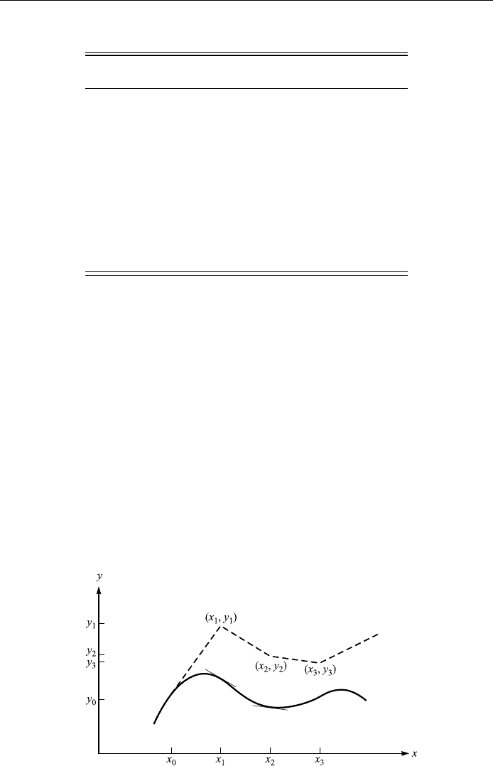
There is a simple geometrical interpretation of Euler's method. We ®rst note
that f x
0
; y
0
y
0
x
0
, and that the equation of the tangent line at the point
x
0
; y
0
to the actual solution curve (or the integral curve) y yx is
y ÿ y
0
Z
x
x
0
f t; ytdt f x
0
; y
0
x ÿ x
0
:
Comparing this with Eq. (13.20), we see that x
1
; y
1
lies on the tangent line to the
actual solution curve at (x
0
; y
0
). Thus, to move from point (x
0
; y
0
) to point (x
1
; y
1
)
we proceed along this tangent line. Similarly, to move to point (x
2
; y
2
we proceed
parallel to the tangent line to the solution curve at (x
1
; y
1
, as shown in Fig. 13.8.
470
NUMERICAL METHODS
The merit of Euler's method is its simplicity, but the successive use of the
tangent line at the approx imate values y
1
; y
2
; ...can accumulate errors. The accu-
racy of the approximate vale can be quite poor, as shown by the following simple
example.
Example 13.4
Use Euler's method to approximate solution to
y
0
x
2
y; y13 on interval 1; 2:
Solution: Using h 0:1, we obtain Table 13.1. Note that the use of a smaller
step-size h will improve the accuracy.
Euler's method can be improved upon by taking the gradient of the integral
curve as the means of obtaining the slopes at x
0
and x
0
h, that is, by using the
471
NUMERICAL SOLUTIONS OF DIFFERENTIAL EQUATIONS
Table 13.1.
xy(Euler) y (actual)
1.0 3 3
1.1 3.4 3.43137
1.2 3.861 3.93122
1.3 4.3911 4.50887
1.4 4.99921 5.1745
1.5 5.69513 5.93977
1.6 6.48964 6.81695
1.7 7.39461 7.82002
1.8 8.42307 8.96433
1.9 9.58938 10.2668
2.0 10.9093 11.7463
Figure 13.8.

approximate value obtained for y
1
, we obtain an improved value, denoted by
y
1
1
:
y
1
1
y
0
1
2
ff x
0
; y
0
f x
0
h; y
1
g: 13:21
This process can be repeated until there is agreement to a required degree of
accuracy between successive approximations.
The three-term Taylor series method
The rationale for this method lies in the three-term Taylor expansion. Let y be the
solution of the ®rst-order ordinary equati on (13.18) for the initial condition
y y
0
when x x
0
and suppose that it can be expanded as a Taylor series in
the neighborhood of x
0
.Ify y
1
when x x
0
h, then, for suciently small
values of h,wehave
y
1
y
0
h
dy
dx
0
h
2
2!
d
2
y
dx
2
ÿ!
0
h
3
3!
d
3
y
dx
3
ÿ!
0
: 13:22
Now
dy
dx
f x; y;
d
2
y
dx
2
@f
@x
dy
dx
@f
@y
@f
@x
f
@f
@y
;
and
d
3
y
dx
3
@
@x
f
@
@y
@f
@x
f
@f
@y
@
2
f
@x
2
@f
@y
@f
@y
2f
@
2
f
@x@y
f
@f
@y
2
f
2
@
2
f
@y
2
:
Equation (13.22) can be rewritten as
y
1
y
0
hf x
0
; y
0
h
2
2
@f x
0
; y
0
@x
f x
0
; y
0
@f x
0
; y
0
@y
;
where we have dropped the h
3
term. We now use this equation as an iterative
equation:
y
n1
y
n
hf x
n
; y
n
h
2
2
@f x
n
; y
n
@x
f x
n
; y
n
@f x
n
; y
n
@y
: 13:23
That is, we compute y
1
yx
0
h from y
0
, y
2
yx
1
h from y
1
by replacing x
by x
1
, and so on. The error in this method is proportional h
3
. A good approxima-
472
NUMERICAL METHODS

tion can be obtained for y
n
by summing a number of terms of the Taylor's
expansion. To illustrate this method, let us consider a very simple example.
Example 13.5
Find the approximate values of y
1
through y
10
for the diÿerential equation
y
0
x y, with the initial condition x
0
1:0 and y ÿ2:0.
Solution: Now f x; yx y;@f =@x @ f =@y 1 and Eq. (13.23) reduces to
y
n1
y
n
hx
n
y
n
h
2
2
1 x
n
y
n
:
Using this simple formula with h 0:1 we obtain the results shown in Table 13.2.
The Runge±Kutta method
In practice, the Taylor series converges slowly and the accuracy involved is not
very high. Thus we often resort to other methods of solution such as the Runge±
Kutta method, which replaces the Taylor series, Eq. (13.23), with the following
formula:
y
n1
y
n
h
6
k
1
4k
2
k
3
; 13:24
where
k
1
f x
n
; y
n
; 13:24a
k
2
f x
n
h=2; y
n
hk
1
=2; 13:24b
k
3
f x
n
h; y
0
2hk
2
ÿ hk
1
: 13:24c
This approximation is equivalent to Simpson's rule for the approximate
integration of f x; y, and it has an error proportional to h
4
. A beauty of the
473
NUMERICAL SOLUTIONS OF DIFFERENTIAL EQUATIONS
Table 13.2.
n x
n
y
n
y
n1
0 1.0 ÿ2.0 ÿ2.1
1 1.1 ÿ2.1 ÿ2.2
2 1.2 ÿ2.2 ÿ2.3
3 1.3 ÿ2.3 ÿ2.4
4 1.4 ÿ2.4 ÿ2.5
5 1.5 ÿ2.5 ÿ2.6

Runge±Kutta method is that we do not need to compute partial derivatives, but it
becomes rather complicated if pursued for more than two or three steps.
The accuracy of the Runge±Kutta method can be improved wi th the following
formula:
y
n1
y
n
h
6
k
1
2k
2
2k
3
k
4
; 13:25
where
k
1
f x
n
; y
n
; 13:25a
k
2
f x
n
h=2; y
n
hk
1
=2; 13:25b
k
3
f x
n
h; y
0
hk
2
=2; 13:25c
k
4
f x
n
h; y
n
hk
3
: 13:25d
With this formula the error in y
n1
is of order h
5
.
You may wonder how these formulas are established. To this end, let us go
back to Eq. (13.22), the three-term Taylor series, and rewrite it in the form
y
1
y
0
hf
0
1=2h
2
A
0
f
0
B
0
1=6h
3
C
0
2f
0
D
0
f
2
0
E
0
A
0
B
0
f
0
B
2
0
Oh
4
; 13:26
where
A
@f
@x
; B
@f
@y
; C
@
2
f
@x
2
; D
@
2
f
@x@y
; E
@
2
f
@y
2
and the subscript 0 denotes the values of these quantities at x
0
; y
0
.
Now let us expand k
1
; k
2
,andk
3
in the Runge±Kutta formula (13.24) in power s
of h in a similar manner:
k
1
hf x
0
; y
0
;
k
2
f x
0
h=2; y
0
k
1
h=2;
f
0
1
2
hA
0
f
0
B
0
1
8
h
2
C
0
2f
0
D
0
f
2
0
E
0
Oh
3
:
Thus
2k
2
ÿ k
1
f
0
hA
0
f
0
B
0
and
d
dh
2k
2
ÿ k
1
h0
f
0
;
d
2
dh
2
2k
2
ÿ k
1
ÿ!
h0
2A
0
f
0
B
0
:
474
NUMERICAL METHODS

Then
k
3
f x
0
h; y
0
2hk
2
ÿ hk
1
f
0
hA
0
f
0
B
0
1=2h
2
fC
0
2f
0
D
0
f
2
0
E
0
2B
0
A
0
f
0
B
0
g
Oh
3
:
and
1=6k
1
4k
2
k
3
hf
0
1=2h
2
A
0
f
0
B
0
1=6h
3
C
0
2f
0
D
0
f
2
0
E
0
A
0
B
0
f
0
B
2
0
Oh
4
:
Comparing this with Eq. (13.26), we see that it agrees with the Taylor series
expansion (up to the term in h
3
) and the formula is established. Formula (13.25)
can be established in a similar manner by taking one more term of the Taylor
series.
Example 13.6
Using the Runge±Kutta method and h 0:1, solve
y
0
x ÿ y
2
=10; x
0
0; y
0
1:
Solution: With h 0:1, h
4
0:0001 and we may use the Runge±Kutta third-
order approximation.
First step: x
0
0; y
0
0; f
0
ÿ0:1;
k
1
ÿ0:1, y
0
hk
1
=2 0:995;
k
2
ÿ0:049; 2k
2
ÿ k
1
0:002; k
3
0;
y
1
y
0
h
6
k
1
4k
2
k
1
0:9951:
Second step: x
1
x
0
h 0:1, y
1
0:9951, f
1
0:001,
k
1
0:001, y
1
hk
1
=2 0:9952;
k
2
0:051, 2k
2
ÿ k
1
0:101, k
3
0:099,
y
2
y
1
h
6
k
1
4k
2
k
1
1:0002:
Third step: x
2
x
1
h 0:2 ; y
2
1:0002, f
2
0:1,
k
1
0:1, y
2
hk
1
=2 1:0052,
k
2
0:149; 2k
2
ÿ k
1
0:198; k
3
0:196;
y
3
y
2
h
6
k
1
4k
2
k
1
1:0151:
475
NUMERICAL SOLUTIONS OF DIFFERENTIAL EQUATIONS