Choudhry. Fixed Income Securities Derivatives Handbook

Подождите немного. Документ загружается.

This page is intentionally blank

293

CHAPTER 16

The Yield Curve, Bond Yield,

and Spot Rates

his chapter examines a number of issues relevant to participants

in the ﬁ xed-income markets. The analysis presented is based on

government-bond trading and is conﬁ ned to generic bonds that

are default-free, with no consideration given to factors that apply to cor-

porate bonds, asset- and mortgage-backed bonds, convertibles, or other

nonvanilla securities, or to issues such as credit risk and prepayment risk.

Nevertheless, the principles adduced are pertinent to all relative-value

ﬁ xed-income analysis.

Practical Uses of Redemption

Yield and Duration

The drawbacks of duration and gross redemption yield (henceforth re-

ferred to simply as yield ) for bond analysis are well documented. That

different bonds, even vanilla government securities, can have their yields

analyzed in a number of ways suggests, moreover, that acceptable return

measures are lacking. When assessing the opportunities available in a mar-

ket, investors often use that market’s yield convention. The resulting mul-

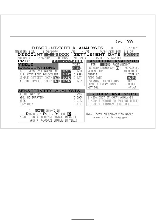
tiplicity of yield-calculation methods—illustrated in

FIGURE 16.1—makes

bond comparisons problematic. Duration is another measure that can be

deﬁ ned in more than one way, again making comparison between differ-

ent bonds difﬁ cult. This section discusses ways to mitigate the problems

inherent in using yield and duration and how using analyses based on

these methods should proceed.

294 Selected Market Trading Considerations

The Concept of Yield

Ideally, an instrument’s yield indicates what return an investor can achieve

by holding it. Such an ideal measure would be a function of the value of

the initial investment, the holding period, and the value of the matured in-

vestment. It would also take into account any reinvestment of the income

received during the holding period—that is, the effect of compounding.

A yield measure having these properties may be deﬁ ned as follows for a

simple instrument such as a Treasury bill.

Consider a T-bill with a term of m days and a price of P. Equation

(16.1) may be rearranged to compute the bill’s true yield, rm.

()

100

(16.1)

where

n = the number of interest periods from value date until maturity

The U.S. Treasury interest basis is semiannual, and the market uses

an actual/actual day count. So, the value of n for the 90-day T-bill

whose yield analysis as of March 25, 2004, is shown in ﬁ gure 16.1

would be 90/183, where 183 represents the number of days in half a

year, given that 2004, as a leap year, had 366 days. The bill was priced

Source: Bloomberg

FIGURE 16.1

Bloomberg YA Screen Showing Alternative Yield

Calculations for a U.S. Treasury

The Yield Curve, Bond Yield, and Spot Rates 295

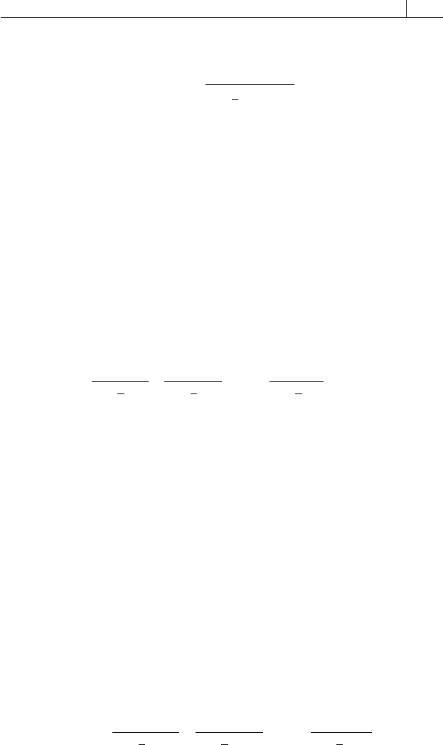
at 99.7725, so its true yield is given by equation (16.2).

99 7725

100

90 183

()

(16.2)

rm = 0.927 percent

The yields quoted on T-bills often differ from their true yields. This

is because their yield calculations often assume simple rather than com-

pound interest. Nevertheless, true yield is important for its application to

longer-dated coupon bonds.

Yield has been deﬁ ned in previous chapters as the discount rate that

equates the sum of the present values of all a bond’s cash ﬂ ows to its ob-

served market price. A vanilla bond, such as a U.S. Treasury, has m future

cash ﬂ ows—the coupon payments—each having a value C, equal to one-

half the coupon rate applied to the face value. C

is the principal payment.

The sum total of the bond’s discounted cash ﬂ ows is given by equation

(16.3).

()

11 1

.....

(16.3)

where

= the i th bond payment

= the coupon payment plus the principal repayment

= the number of days from the value date to maturity

= the number of interest periods from the value date until C

= m

182 or 183

r = the discount rate

From this it is easy to derive the deﬁ nition of true yield, which is the

discount rate that equates a bond’s current market price to the present

value of its cash ﬂ ows. The bond’s market price is its dirty price—that is,

the price including accrued interest. This is represented in (16.4), where

PV is replaced by P, representing the clean price plus AI, representing

accrued interest.

PAI

()

11 1

.....

(16.4)

296 Selected Market Trading Considerations

Yield Comparisons in the Market

U.S. Treasury price quotes are in ticks, or thirty-seconds of a price point.

A half tick is denoted by a plus sign. On May 10, 1994, the 10.25 per-

cent Treasury bond maturing July 21, 1995, was quoted at 104-28+—

in other words, an investor would pay $104.28625 for every $100 in

face value. It pays coupons on January 21 and July 21. On May 11,

1994, the settlement date, it will have accrued 109 days of interest, for a

total of 10.25 × 109/365 × 0.5, or 1.53048 for every $100 of face value.

The dirty price of the bond on this date is thus 104-28+ plus 1.53048,

or 106.421105.

The remaining bond cash ﬂ ows are $5.125, on both July 21, 1994,

and January 21, 1995, and $105.25, on July 21, 1995. January 21, 1995,

however, is a Saturday, so the cash ﬂ ow will not actually be received until

Monday, January 23. The number of days between the value date, May

11, 1994, and the receipt of each cash ﬂ ow is

July 21, 1994 71 days

January 23, 1995 230 days

July 21, 1995 436 days

The interest periods between each cash ﬂ ow date and the value date

number are

(71/183) or 0.387978

(230/183) or 1.256830

(436/183) or 2.382513

Plugging the derived values for price, accrued interest, cash ﬂ ows, and

interest periods into (16.4) gives

106 421105

5 125

105

0 387978

1 256830

()

rm rm

125

2 38251

()

which can be rearranged to solve for rm = 0.073894, or 7.3894 per-

cent.

The conventional yield—the one usually quoted—is almost invari-

ably different from the true yield. This is because the conventional cal-

culation derives the number of interest periods between the value date

and the cash ﬂ ows based on exact half-year intervals between payments,

ignoring the delays that occur when the payment dates fall on nonbusi-

ness days.

The Yield Curve, Bond Yield, and Spot Rates 297

Measuring a Bond’s True Return

The true yield measure derived in the previous section is not as straight-

forward as the one given earlier for the T-bill. Because a T-bill has only a

single cash ﬂ ow, its maturity value is known, so its return is easily calculat-

ed as its increase in value from start to maturity. Investors know that mon-

ey put into a 90-day T-bill with a yield of 5 percent will have grown by

5 percent, compounded semiannually, at the end of three months. No such

certainty is possible with coupon-bearing bonds. Consider: although the

investors in the 90-day T-bill are assured of a 5 percent yield after ninety

days, they don’t know what their investment will be worth after, say, sixty

days or at what yield they will be able to reinvest their money when the bill

matures. Such uncertainties don’t effect the return of the short-term bill,

but they have a critical impact on the return of coupon bonds.

It would certainly help investors if they could analyze bonds as though

they had single cash ﬂ ows. Investors often buy bonds against liabilities that

they must discharge on known future dates. It would be a comfort if they

could be sure the bonds’ returns would meet their liability requirements.

Put very simply, this is the concept of immunization.

The difﬁ culty in calculating a bond’s return is that its future value is

not known with certainty, because it depends on the rates at which the

interim cash ﬂ ows can be reinvested, and these rates cannot be predicted.

A number of approaches have been proposed that get around this. These

are described in the following paragraphs, assuming simple interest rate

environments.

The simplest approach assumes, somewhat unrealistically, that the

yield curve is ﬂ at and moves only in parallel shifts, up or down. It con-

siders a bond to be a package of zero-coupon securities whose values are

discounted and added together to give its theoretical price. The advantage

of this approach is that each cash ﬂ ow is discounted at the interest rate for

the relevant term, rather than at a single “internal rate of return,” as in the

conventional approach. Given the ﬂ at yield curve, however, this approach

reduces to (16.3). An example of its application is on the following page.

A bond’s return is inﬂ uenced by changes in the yield curve that occur

after its purchase. Say the yield curve moves in a parallel shift to a new level,

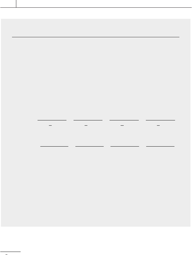
. In that case, the expected future value of the bond changes. Assuming

s interest periods from the value date to a speciﬁ ed “horizon date,” the new

value of the bond on that horizon date is given by equation (16.5).

(16.5)

Prm s

11 1

, .....

()

−

−−

()

−

()

−

298 Selected Market Trading Considerations

The equation expresses the fact that the C

m–i

cash ﬂ ow contributes

)

−

to the bond’s value on this future horizon date. If this cash

ﬂ ow is received ahead of the horizon date,

−

is a negative exponent,

meaning that C

is compounded (rather than discounted) forward to the

horizon date at the rate rm

. If the cash ﬂ ow is received after the horizon

date,

−

is positive, and C

is discounted back to the horizon date at

the same rate.

If s is small, a majority of the bond’s cash ﬂ ows take place after the

horizon date, and a shift up in the yield curve—that is, rm

> rm—

produces a lower future value,

Prm s

()

, because most of the ﬂ ows must

be discounted at the higher rate. If s is large, so that most of the cash ﬂ ows

take place before the horizon date, an upward shift increases the value of

these cash ﬂ ows, because they can be reinvested at a higher rate of inter-

est. When s is sufﬁ ciently large, this reinvestment gain matches, and may

EXAMPLE: Conventional Bond Pricing

Given a value date of December 8, 2000, value a hypotheti-

cal bond paying a 5 percent semiannual coupon and maturing

December 8, 2002.

On the value date, the bond has precisely four interest periods

to maturity and no accrued interest. Its cash ﬂ ows are 2.50, 2.50,

2.50, and 102.50. Assuming that the yield curve on December 7

is ﬂ at at 5 percent, its price is calculated as follows:

PAI

nnnn

()

1111

1234

2.50

1 0.025

()

123

250

1 0 025

250

1 0 025

10.

2250

1 0 025

2 4390 2 3879 2 3215 92 8600

... .

()

=+++

100.00=

So, at a uniform—because of the ﬂ at curve—discount rate of

5 percent, the price of the bond is par.

The Yield Curve, Bond Yield, and Spot Rates 299

even exceed, the loss suffered through revaluation of the discounting at the

higher rate, resulting in a higher future value,

Prm s

()

. The reverse occurs

rm rm

. These changes in future value represent the reinvestment risk

borne by the bondholder.

Between the short- and long-term horizon dates is one at which the

net effect of the change in reinvestment rate on the bond’s future value

is close to zero. At this date, the bond behaves like a single-cash-ﬂ ow or

zero-coupon security, and its future value can be predicted with greater

certainty, no matter what the yield curve does after its purchase. Deﬁ n-

ing this date as s

interest periods after the purchase date and P

as the

value of the bond at that point, it can be shown that the bond’s rate of

return up to this horizon date is the value for rm

that solves equation

(16.6).

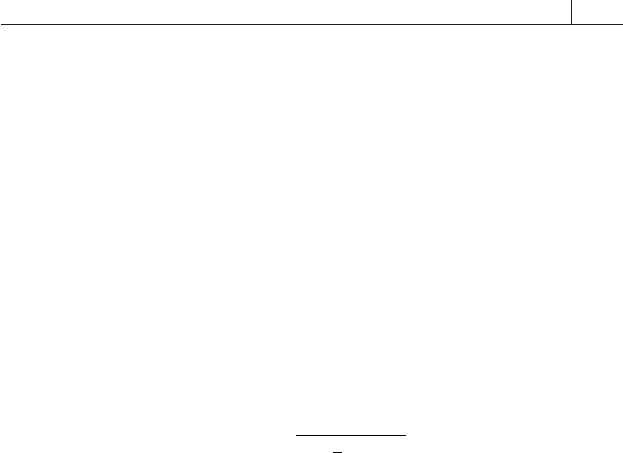
PAI

()

(16.6)

The left side of equation (16.6) is the bond’s market price broken

into clean price plus accrued interest, as it was in (16.4). In fact, it can be

shown that rm

is identical to the initial yield in (16.4), rm. The value of

that results in a stable future bond value is the Macaulay duration. At

this point, assuming the existence of only one, parallel yield shift, a change

in yield will not impact the future value of the bond. The bond’s cash ﬂ ows

are immunized, and the instrument can be used to match a liability exist-

ing on that date.

Because of the analysis’s assumed restrictions, however, investors apply-

ing it must continually adjust their portfolios if they wish to remain im-

munized. Fabozzi (1996) contains a very accessible discussion of the key

issues involved in dynamically managing a portfolio. A number of other

considerations also limit the use of duration in portfolio management.

For instance, as Blake (1990) 5.8.1 points out, most Treasury bonds have

durations of less than twelve years. This makes portfolio immunization

difﬁ cult when liabilities are very long dated.

Zero-coupon bonds don’t pose these problems, because their durations

are identical to their terms to maturity. This potentially increases their at-

tractiveness as investments. A ﬁ ve-year zero-coupon bond has a duration

of ﬁ ve years when purchased; after two years, its duration is three years, no

matter what interest rates have done. A long-dated zero-coupon bond can

thus be safely used to match a long-dated liability.

300 Selected Market Trading Considerations

Implied Spot Rates and

Market Zero-Coupon Yields

The yield analysis described above considers coupon bonds as packages

of zeros. How does one compare the yields of zero-coupon and coupon

bonds? A two-year zero is clearly the point of comparison for a coupon

bond whose duration is two years. What about very long-dated zero-

coupon bonds, though, for which no equivalent coupon Treasury is usu-

ally available? The solution lies in the technique of stripping coupon

Treasuries, which allows implied zero-coupon rates to be calculated, which

can be compared with actual strip-market yields.

This section describes the relationships among spot interest rates and

the actual market yields on zero-coupon and coupon bonds. It explains

how an implied spot-rate curve can be derived from the redemption yields

and prices observed on coupon bonds, and discusses how this curve may

be used to compare bond yields. Note that, in contrast with the common

practice, spot rates here refer only to rates derived from coupon-bond

prices and are distinguished from zero-coupon rates, which denote rates

actually observed on zero-coupon bonds trading in the market.

Spot Yields and Coupon-Bond Prices

As noted in chapter 2, a Treasury bond can be seen as a bundle of individual

zero-coupon securities, each maturing on one of the bond’s cash ﬂ ow pay-

ment dates. In this view, the Treasury’s price is the sum of the present values

of all the constituent zero-coupon bond yields. Assume that the spot rates

for the relevant maturities—

rrr r

N123

, , ,....

—can be observed. If a bond pays

a semiannual coupon computed at an annual rate of C from period 1 to

period N, its present value can be derived using equation (16.7).

(16.7)

()

−

.....

2 100

()

−N

Equation (16.7) differs from the conventional redemption yield for-

mula in that every cash ﬂ ow is discounted, not by a single rate, but by the

zero-coupon rate corresponding to the maturity period of the cash ﬂ ow.

To apply this equation, the zero-coupon-rate term structure must be

known. These rates, however, are not always readily observable. Treasury

prices, on the other hand, are and can be used to derive implied spot in-

terest rates. (Although in the market the terms are used interchangeably,

from this point on, zero coupon will be used only of observable rates and

The Yield Curve, Bond Yield, and Spot Rates 301

spot only of derived ones.) To see how the derivation works, consider the

ten hypothetical U.S. Treasuries whose maturities, prices, and yields are

shown in

FIGURE 16.2. Assume that the yield curve is positive and that the

securities’ settlement date—March 1, 1999—is a coupon date, so none of

them has accrued interest.

The ﬁ rst bond matures in precisely six months and thus has no inter-

mediate cash ﬂ ow before redemption. It can therefore be treated as a zero-

coupon bond, and its yield of 6 percent taken as the 6-month spot rate.

Using this, the 1-year spot rate can be derived from the price of a 1-year

coupon Treasury. The principle of no-arbitrage pricing requires that the

price of a 1-year Treasury strip equal the sum of the present value of the

coupon Treasury’s two cash ﬂ ows:

September 1, 1999 $5

March 1, 2000 $5 + $100 = $105

The combined present values of these cash ﬂ ows is given by equation

(16.8).

FIGURE 16.2 Ten Hypothetical Treasuries

MATURITY YEARS TO COUPON YIELD TO

DATE MATURITY (%) MATURITY PRICE

1-Sep-99 0.5 5.0 6.00 99.5146

1-Mar-00 1.0 10.0 6.30 103.5322

1-Sep-00 1.5 7.0 6.40 100.8453

1-Mar-01 2.0 6.5 6.70 99.6314

1-Sep-01 2.5 8.0 6.90 102.4868

1-Mar-02 3.0 10.5 7.30 108.4838

1-Sep-02 3.5 9.0 7.60 104.2327

1-Mar-03 4.0 7.3 7.80 98.1408

1-Sep-03 4.5 7.5 7.95 98.3251

1-Mar-04 5.0 8.0 8.00 100.0000